Monte Carlo neutrino oscillations (original) (raw)
Abstract
We demonstrate that the effects of matter upon neutrino propagation may be recast as the scattering of the initial neutrino wavefunction. Exchanging the differential, Schrodinger equation for an integral equation for the scattering matrix S permits a Monte Carlo method for the computation of S that removes many of the numerical difficulties associated with direct integration techniques.
Figures (8)
[
Equation (@) allows us to change the independent vari- able from x to ¢ and so measure distances in terms of this quantity. We see that ¢ has a physical interpreta- tion as the number of half periods of the purely adiabatic solutions (ie. 6’ = 0) of the Schrodinger equation (i). Substitution of these definitions into equation () pro- duces where I is the related to the adiabaticity parameter, Note that this definition indicates that a wavefunction will evolve non-adiabaticly if [ >> 1. The change in basis allows us to focus the problem on the non-adiabatic part of the solution by which we mean that portion that jumps from one matter eigenstate to the other because, in this new basis, the Schrodinger equation is now purely off-diagonal. By integrating equation (9) we obtain
[
FIG. 1: The absolute value of the inverse adiabaticity param- eter [ as a function of the period counting variable ¢. The density profile is the BS2005-AGS,OP Standard Solar Model and we selected 6m? = 3 x 10⁷° eV”, E = 10 MeV. In the top panel we used sin?(2 6y) = 0.001 and for the bottom sin?(20v) = 0.1.
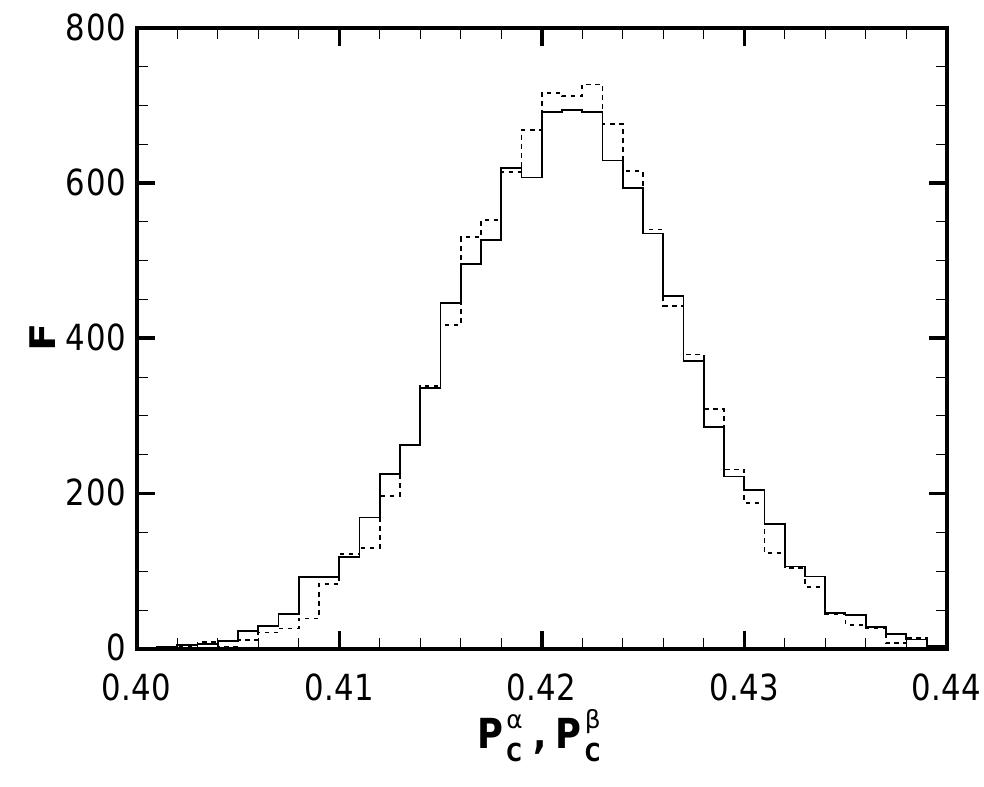
FIG. 2: The frequency distribution of Pg (solid) and PS (dashed) of 10,000 results from the Monte Carlo calcula- tion using the BS2005-AGS,OP Standard Solar Model 3h, 6m? = 3 x 10⁷° eV”, E = 10 MeV and sin?(26y-) = 0.001 as the physical parameters. The number of trials is Nr = 10%.
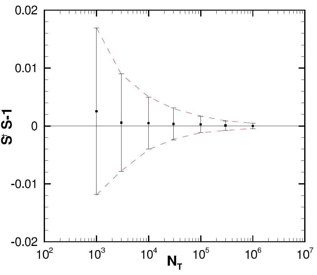
FIG. 3: The mean value of St S$ — 1 indicated by the squares as a function of Nr for the calculation outlined in the text. The error bars are not the error in the mean but rather indi- cate the 1 —o spread in the values of S'S — 1. The dashed lines are StS —14C/V/Nr with C = 0.468.
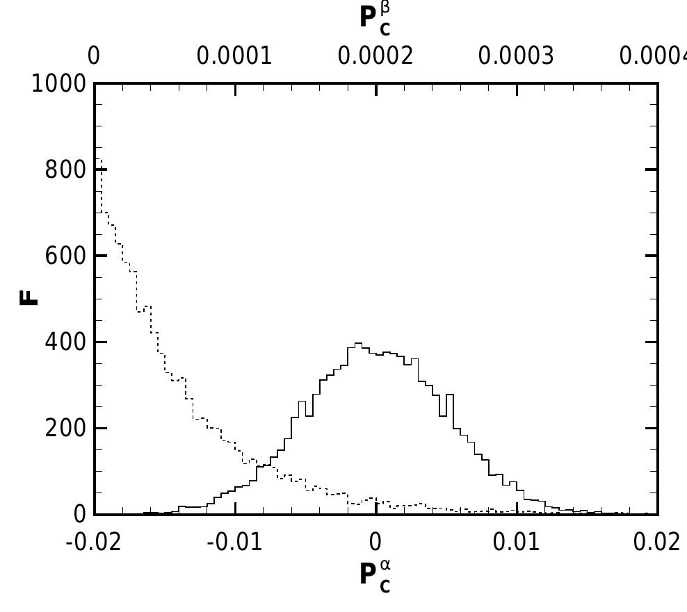
FIG. 4: The frequency distribution of P§ (solid) and P& (dashed) of 10,000 results from the Monte Carlo calcula- tion using the BS2005-AGS,OP Standard Solar Model 3h, dm? = 3 x 10~-° eV’, E = 10 MeV and sin?(26v) = 0.1 as the physical parameters. The number of trials is again Nr = 10%.
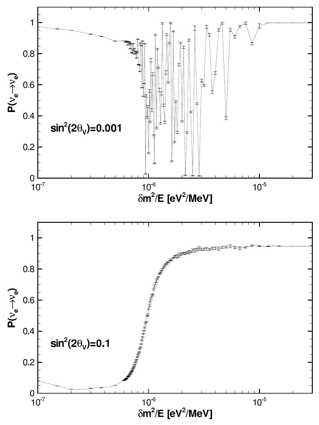
FIG. 5: The neutrino survival probability through the Stan- dard Solar Model density profile as a function of 6m?/E. In the top panel sin?(26y-) = 0.001, in the bottom sin?(26y) = 0.1. The source of neutrinos is located at 3/10 Ro and the neutrinos propagate back through the core and out the other side. The error bars on each point are the rms spread in the results from 8 repetitions. The Gaussian estimator leads to a bias so the accuracy should be regarded as illustrative.
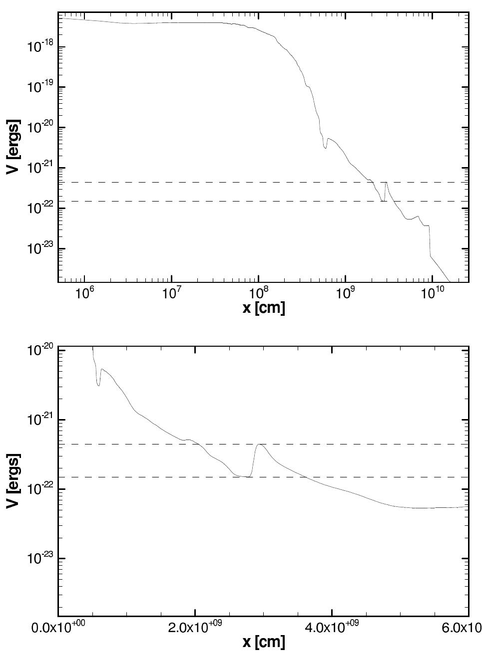
FIG. 6: The electron neutrino potential energy, V = /2E FNe, as a function of radial distance for the model dis- cussed in the text. The upper figure is the entire profile, the lower focuses upon that portion up to 6x 10° cm. In both pan- els the dashed lines indicate the resonance potential energies for 5.4 MeV (upper) and 16 MeV (lower) neutrinos indicating that neutrinos with energies between these values will expe- rience a triple resonance. The mass splitting is chosen to be dm? = 3 x 10⁷% eV? and sin?(26y) = 4 x 1074.
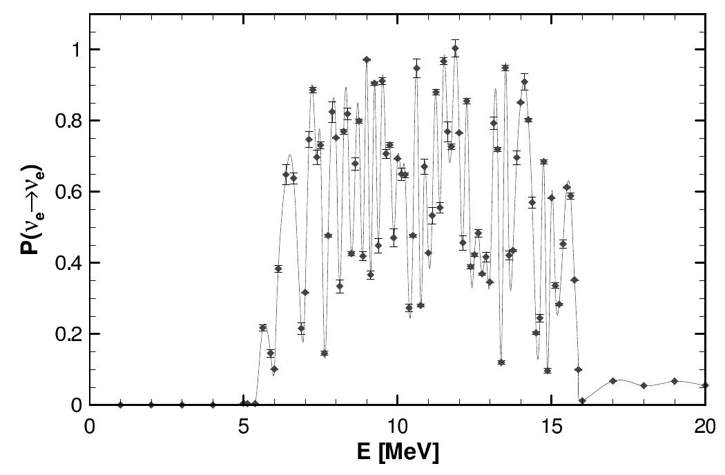
FIG. 7: The neutrino survival probability through the density profile shown in figure (@) as a function of the neutrino energy. For this calculation 6m? = 3 x 1073 eV? and sin?(20v) = 4x 10-*. Again, the error bars on each point are the rms spread in the results from 8 repetitions of the calculation using the Gaussian estimator. Though this estimator is biased they indicate the accuracry of the result.

Loading Preview
Sorry, preview is currently unavailable. You can download the paper by clicking the button above.
References (24)
- S.P. Mikheev and A.I. Smirnov, Nuovo Cimento C, 9, 17, (1986)
- L. Wolfenstein, Phys. Rev., D17, 2369 (1978)
- Q. R. Ahmad et al. [SNO Collaboration], Phys. Rev. Lett. 89, 011301 (2002) [arXiv:nucl-ex/0204008].
- H.A. Bethe, Physical Review Letters, 56, 1305 (1986)
- W.C. Haxton, Physical Review Letters, 57, 1271 (1986)
- I. Mocioiu and R. Shrock, Phys. Rev. D 62, 053017 (2000) [arXiv:hep-ph/0002149].
- G. M. Fuller, W. C. Haxton and G. C. McLaughlin, Phys. Rev. D 59, 085005 (1999) [arXiv:astro-ph/9809164].
- A. S. Dighe and A. Y. Smirnov, Phys. Rev. D 62, 033007 (2000) [arXiv:hep-ph/9907423].
- L.R. Petzold, Siam J. Numer. Anal., 18, 455 (1981)
- R.C. Schirato, and G.,M. Fuller, astro-ph/0205390
- J. Engel, G.C. McLaughlin, and C. Volpe, Phys.Rev. D67, 013005 (2003)
- C. Lunardini and A. Y. Smirnov, JCAP 0306, 009 (2003) [arXiv:hep-ph/0302033].
- M. Kachelrieß, and R. Tomàs, Phys. Rev. D , 64, 073002 (2001)
- A. Friedland, Phys. Rev. D , 64, 013008 (2001)
- H.W. Lilliefors, Journal of the ASA, 62, 399 (1967)
- W.C. Haxton, Phys. Rev. D , 35, 2352 (1987)
- T.K. Kuo, and J. Pantaleone, Reviews of Modern Physics, 61, 937 (1989)
- A.B. Balantekin, and J.F. Beacom, Phys.Rev., D54, 6323 (1996)
- F.N. Loreti, and A.B. Balantekin, Phys.Rev. D50, 4762 (1994)
- F.N. Loreti, et al., Phys. Rev. D , 52, 6664 (1995)
- A.B. Balantekin, J.M. Fetter, and F.N. Loreti, Phys.Rev., D54, 3941 (1996)
- P.M. Fishbane, and P. Kaus, Journal of Physics G, 27, 2405 (2001)
- J.N. Bahcall, and A.M. Serenelli, and S. Basu, Ap. J. L., 621, L85 (2005)
- J. Blondin, J. Brockman,, J.P. Kneller, and G.C. McLaughlin, in preparation