Customer Demand Forecasting via Support Vector Regression Analysis (original) (raw)
Abstract
T his paper presents a systematic optimization-based approach for customer demand forecasting through support vector regression (SVR) analysis. The proposed methodology is based on the recently developed statistical learning theory (Vapnik, 1998) and its applications on SVR. The proposed three-step algorithm comprises both nonlinear programming (NLP) and linear programming (LP) mathematical model formulations to determine the regression function while the final step employs a recursive methodology to perform customer demand forecasting. Based on historical sales data, the algorithm features an adaptive and flexible regression function able to identify the underlying customer demand patterns from the available training points so as to capture customer behaviour and derive an accurate forecast. The applicability of our proposed methodology is demonstrated by a number of illustrative examples.
Figures (16)
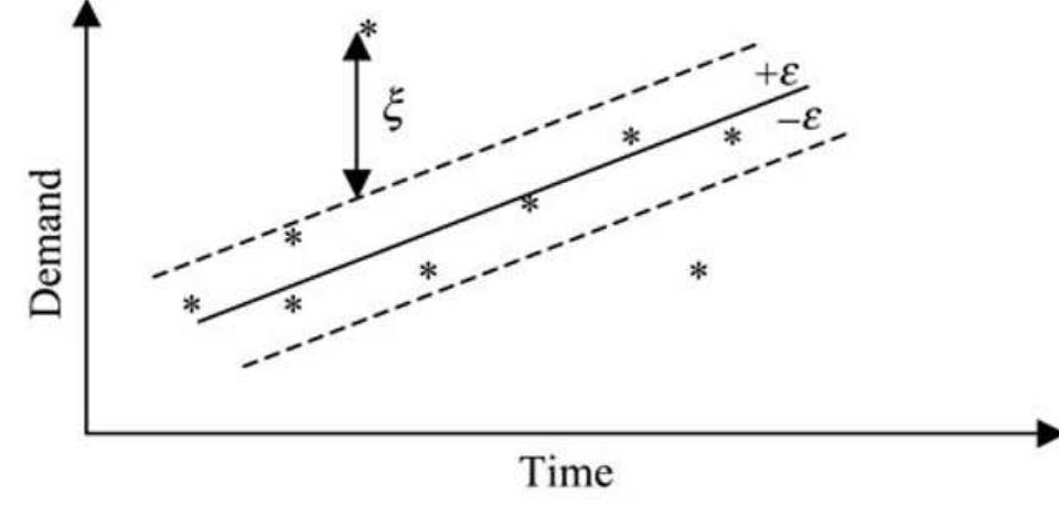
Figure 1. Graphical representation of support vector regression (* depicts training points).
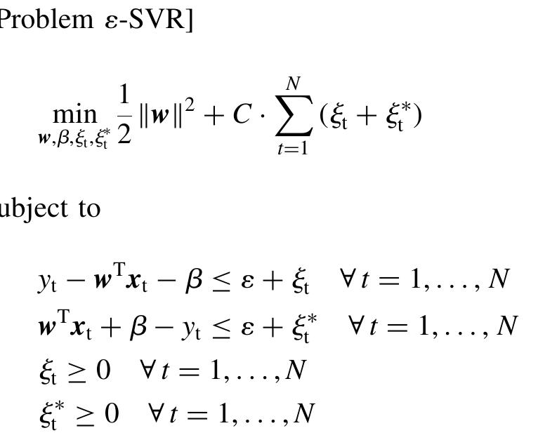
Overall, the SVR analysis takes the form of the following constrained optimization problem (Vapnik, 1998): The first term in the objective function represents model complexity (flatness) while the second term represents the model accuracy (error tolerance). The parameter C is a positive scalar determining the trade-off between flatness and error tolerance (regularization parameter), while &, and &* represent the absolute deviations above and below the e-insensitive tube.
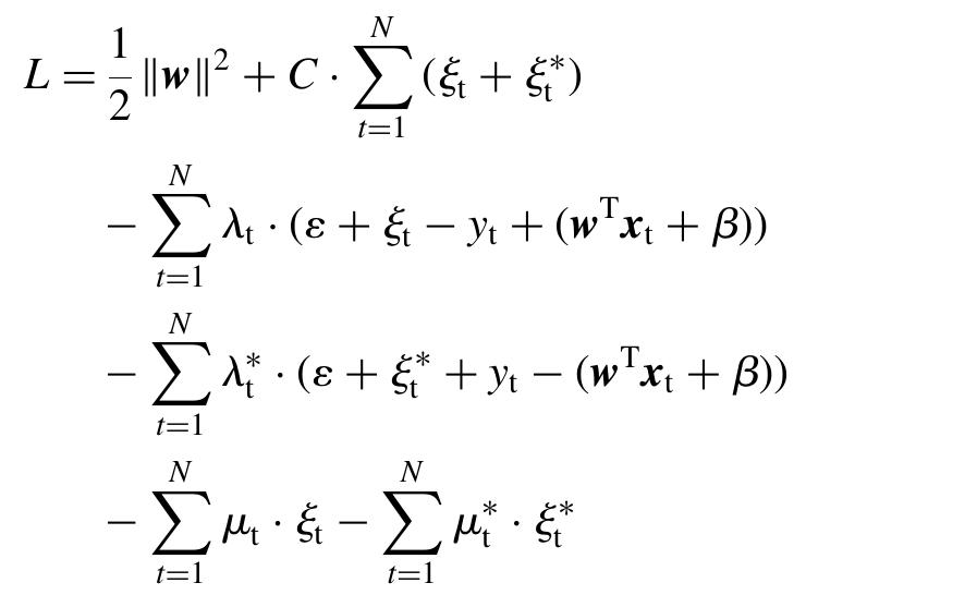
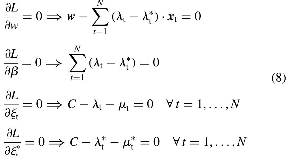
At the optimal point Karush—Kuhn—Tucker (KKT) conditions impose that the partial derivatives of L with respect to the primal variables (w, B, &, &) equal zero: We can easily construct the Lagrangean function of the primal problem by bringing all constraints into the objec- tive function with the use of appropriately defined Lagrange multipliers 44, AS b, we as follows:
By substituting equations (8) into (7), we obtain the dual optimization problem:
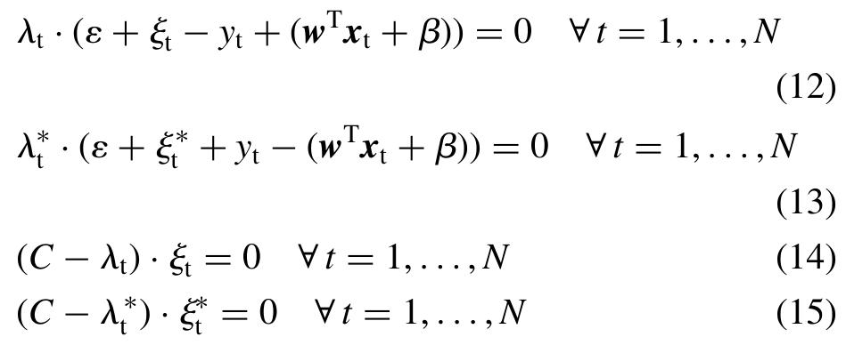
Parameter 6 can be calculated from the KKT complemen- tarity conditions which state that the product between dual variables and constraints has to vanish as follows: According to the aforementioned KKT complementarity conditions, training points lying outside the e-insensitive tube have A, =C (or Aj =C) and & #40 (or & # 0). Those points are called support vectors. Furthermore, there exists no set of dual vaiariables A, and A which are both nonzero simultaneously as this would require nonzero slack variables in both directions. Finally, training points within the e-insensitive tube have A,€&(0,C) (or Ay € (0, C)) and also & =0 (or &*=0) (Smola and Scholkopf, 1998).
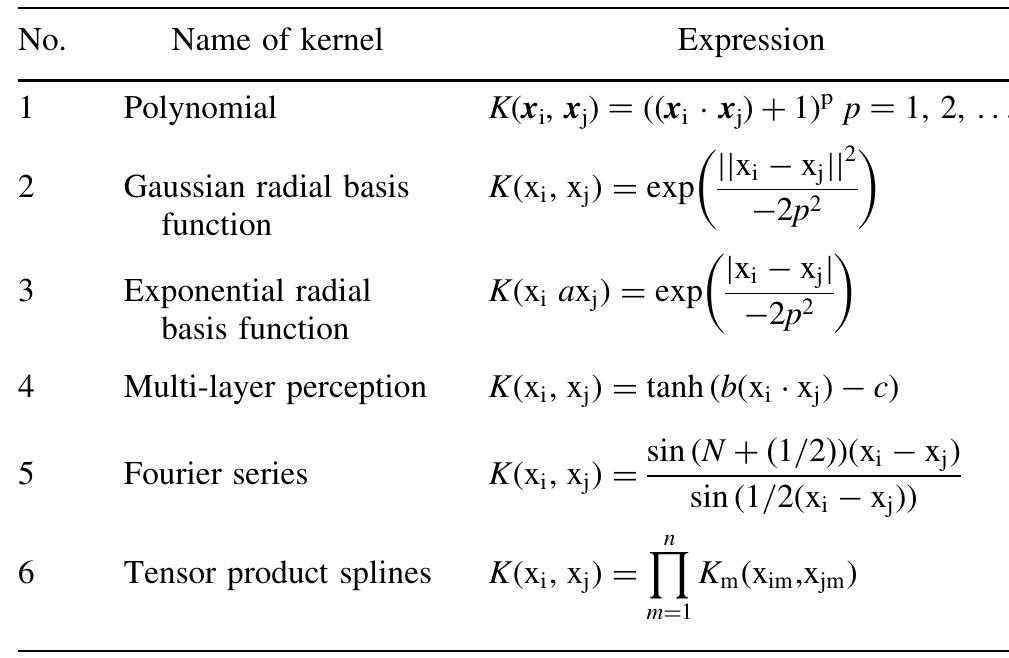
Table 1. Different types of kernel functions. Any function satisfying Mercer’s theorem (Mercer, 1909) may be employed as a kernel function. The types of functions most commonly used in SVM literature as kernel functions are summarized in Table 1 (see for example, Kulkarni et al., 2004).
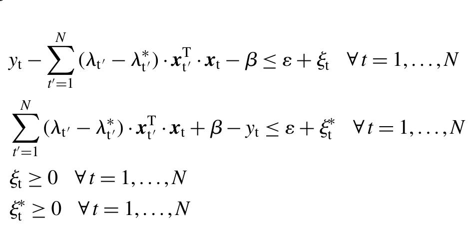
The solution of Problem P derives simultaneously the values for both 6 and variables & and &. It is worth men- tioning that A, and Af are now treated as parameters whose values are given from the solution of the dual problem solved earlier on. Notice also that Problem P is a simple linear programming (LP) model and therefore it can be solved with great computational efficiency even for large number of training points.
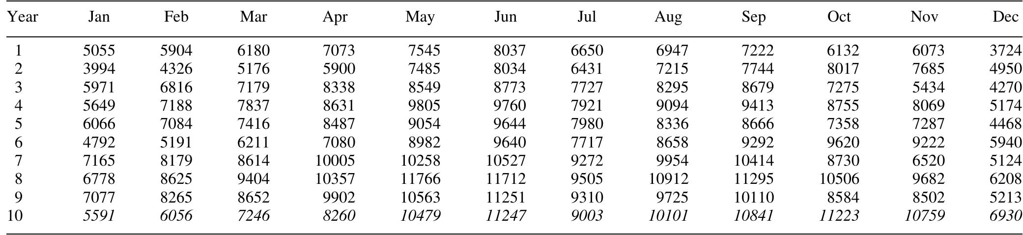
Table 5. Monthly chemical sales (in tonnes). Trans IChemE, Part A, Chemical Engineering Research and Design, 2005, 83(A8): 1009-1018
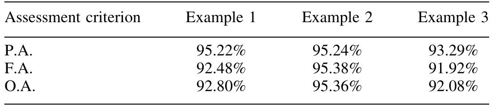
Table 4. Forecasting assessment criteria for the illustrative examples.
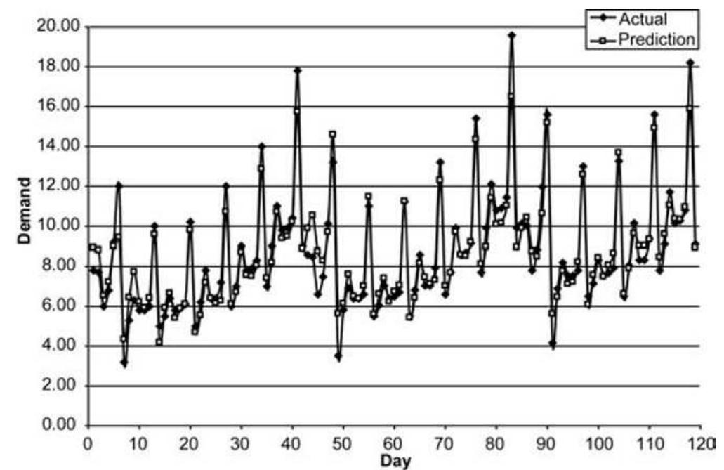
Figure 2. Customer demand forecast for example 1.
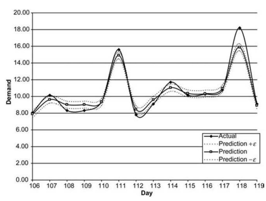
Figure 3. Focus on customer demand forecast for example 1.
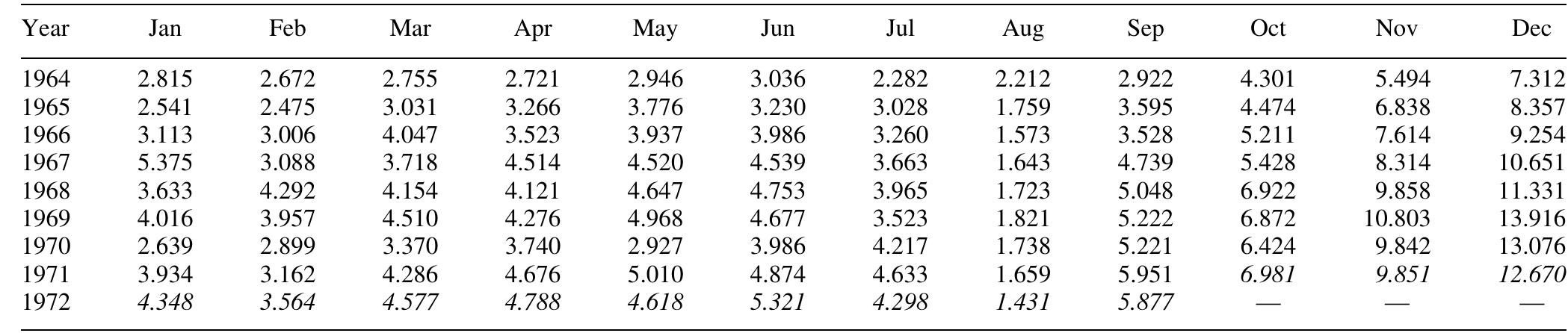
Table 6. Monthly champagne sales—France (millions of bottles). Trans IChemE, Part A, Chemical Engineering Research and Design, 2005, 83(A8): 1009-1018
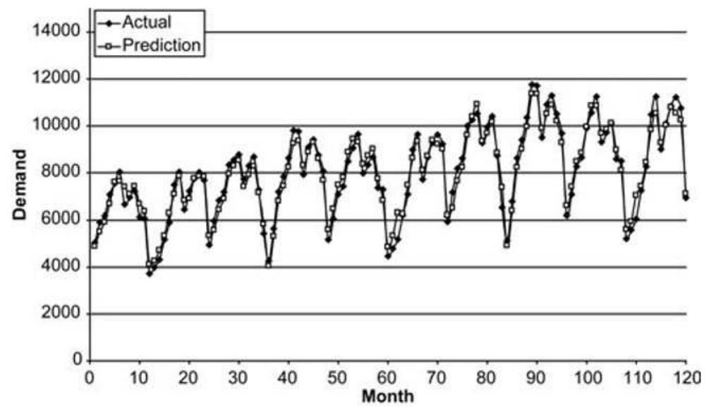
Figure 4. Customer demand forecast for example 2.
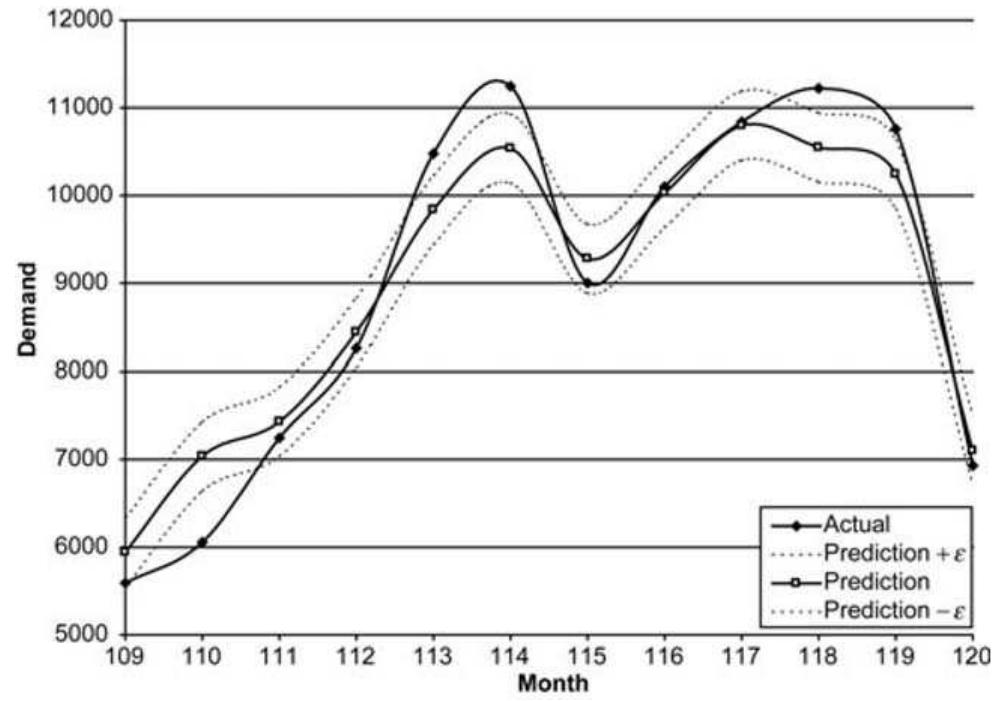
Figure 5. Focus on customer demand forecast for example 2.
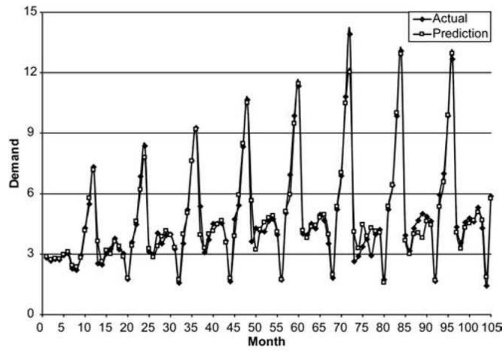
Figure 6. Customer demand forecast for example 3.
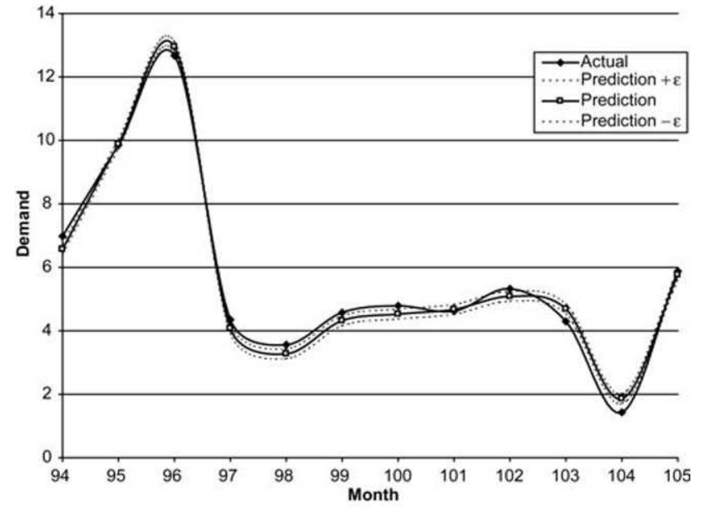
Figure 7. Focus on customer demand forecast for example 3. SVR analysis. Historical customer demand patterns were used as training points attributes for the SVR. The proposed approach employed a three-step algorithm in order to extract information from the training points and identify an adaptive basis regression function before it performs a recursive methodology for customer demand forecasting. The applicability of the proposed forecasting approach was then validated through a number of illustrative custo- mer demand forecasting examples. In all three examples, the proposed methodology handled successfully complex nonlinear customer demand patterns and derived forecasts with prediction accuracy of more than 93% in all cases. Although, future work should consider a formal way of determining SVR parameters, support vector regression can still be regarded as a parsimonious alternative to com- plex artificial neural networks forecasting.

Loading Preview
Sorry, preview is currently unavailable. You can download the paper by clicking the button above.
References (27)
- Agrawal, M., Jade, A.M., Jayaraman, V.K. and Kulkarni, B.D., 2003, Sup- port vector machines: a useful tool for process engineering applications, Chem Eng Prog, 99: 57-62.
- Aizerman, M.A., Braverman, E.M. and Rozoner, L.I., 1964, Theoretical foundations of the potential function method in pattern recognition learning, Automation and Remote Control, 25: 821-837.
- Bhat N.V. and McAvoy, T.J., 1992, Determining model structure for neural models by network stripping, Comput Chem Eng, 16: 271-281.
- Bertsekas, D.P., 1995, Nonlinear Programming (Athena Scientific, Massachusetts, USA).
- Box, G.E.P. and Jenckins, G.M., 1969, Time Series Analysis, Forecasting and Control (Holden-Day, San Francisco, USA).
- Brooke, A., Kendrick, D., Meeraus, A. and Raman, R., 1998, GAMS: A User's Guide (GAMS Development Corporation, Washington, USA).
- Burges, C.J.C., 1998, A tutorial on support vector machines for pattern recognition, Data Mining and Knowledge Discovery, 2: 121-167.
- Chalimourda, A., Scholkopf B. and Smola A.J., 2004, Experimetally optimal v in support vector regression for different noise models and parameters settings, Neural Networks, 17: 127-141.
- Chang, C.-C. and Lin C.-J., 2001, LIBSVM: a library for support vector machines, software available at http://www.csie.ntu.edu.tw/cjlin/ libsvm.
- Cherkassky, V. and Ma, Y.Q., 2004, Practical selection of SVM par- ameters and noise estimation for SVM regression, Neural Networks, 17: 113-126.
- Cherkassky, V. and Mulier, F., 1998, Learning From Data: Concepts, Theory and Methods (John Wiley and Sons, New York, USA).
- Chiang, L.H., Kotanchek, M.E. and Kordon, A.K., 2004, Fault diagnosis based on Fisher discriminant analysis and support vector machines, Comput Chem Eng, 28: 1389-1401.
- Foster, W.R., Collopy, F. and Ungar, L.H., 1992, Neural network forecast- ing of short noisy time series, Comput Chem Eng, 16: 293-297.
- Floudas, C.A., 1995, Nonlinear and Mixed-Integer Optimization: Funda- mentals and Applications (Oxford University Press Inc., New York, USA).
- Gunn, S.R., 1998, Support Vector Machines for Classification and Regression, Technical Report, Faculty of Engineering, Science and Mathematics, School of Electronics and Computer Science, University of Southampton, UK.
- Kulkarni, A., Jayaraman, V.K. and Kulkarni, B.D., 2004, Support vector classification with parameter tuning assisted by agent-based technique, Comput Chem Eng, 28: 311-318.
- Lasschuit, W. and Thijssen, N., 2004, Supporting supply chain planning and scheduling decision in the oil and chemistry industry, Comput Chem Eng, 28: 863-870.
- Levis, A.A. and Papageorgiou, L.G., 2004, A hierarchical solution approach for multi-site capacity planning under uncertainty in the pharmaceutical industry, Comput Chem Eng, 28: 707-725.
- Makridakis, S. and Hibon, M., 1979, Accuracy of forecasting: an empirical investigation, J Roy Statistical Society A, 142: 97-125.
- Makridakis, S. and Wheelwright, S.C., 1978; Interactive Forecasting: Univariate and Multivariate Methods (Holden-Day Inc., San Francisco, USA).
- Makridakis, S. and Wheelwright, S.C., 1982, The Handbook of Forecasting: A Manager's Guide (John Wiley and Sons, New York, USA).
- Maravelias, C.T. and Grossmann, I.E., 2001, Simultaneous planning for new product development and batch manufacturing facilities, Ind Eng Chem Res, 40: 6147-6164.
- Mercer, J., 1909, Functions of positive and negative type and their connec- tion with the theory of integral equations, Philos Trans Roy Soc London A, 209: 415-446.
- Myasnikova, E., Samsonova, A., Samsonova, M. and Reinitz, J., 2002, Support vector regression applied to the determination of the develop- mental age of a Drosophila embryo from its segmentation gene expression patterns, Bioinformatics, 18: S87-S95.
- Prakasvudhisarn, C., Trafalis, T.B. and Raman, S., 2003, Support vector regression for determination of minimum zone, J Manuf Sci Eng, 125: 736-739.
- Smola, A.J. and Scholkopf, B., 1998, A Tutorial on Support Vector Regression, NeuroCOLT2 Technical Report Series, available from website: http://www.neurocolt.com.
- Vapnik, V.N., 1998, Statistical Learning Theory (John Wiley and Sons, New York, USA). The manuscript was received 26 August 2004 and accepted for publi- cation after revision 6 June 2005. Figure 7. Focus on customer demand forecast for example 3.