Exact Solution of Space-Time Fractional Partial Differential Equations by Adomian Decomposition Method (original) (raw)
Abstract
The intention behind this paper is to achieve exact solution of one dimensional nonlinear fractional partial differential equation(NFPDE) by using Adomian decomposition method(ADM) with suitable initial value. These equations arise in gas dynamic model and heat conduction model. The results show that ADM is powerful, straightforward and relevant to solve NFPDE. To represent usefulness of present technique, solutions of some differential equations in physical models and their graphical representation are done by MATLAB software.
Figures (8)

Taking term by term comparison on both side of equation (3.7), we set recursion scheme like: and so forth. Wherever every component can be determined by manipulating the preceding components and we can attain the solution in a series form by computing the components un(za, t),n > 0. Eventually, we approximate the solution u(x,t) by the reduced series. Then the solution u(z, t) of IVP (3.1) — (3.2) is

where A,and B,, are the Adomian polynomials to be determined from the nonlinear term uDfu and u’ . Comparing both side of equation (4.5) we have

Fig. 1. 2D Graphical representation of solution (4.6) of IVP (4.1)-(4.2) for different values of a such as a = 1,0.8,0.6,0.4 and exact when x = 0.25. Fig. 1 is the graphical behaviour of ADM solution (4.6) for different values of a such as a = 1, 0.8, 0.6, 0.4 and exact solution (4.7) when « = y = 0.25. Figs. 2(a),(b) and 3(c), (d) shows the surface of the 4 terms of the improved ADM solution (4.6) for values of a = 1,0.8,0.6 and surface of exact solution (4.7). It is clear from Fig. 1 and Figs. 2 to 3, in the limit while a > 1, (4.6) approaches to the exact solution (4.7). Fig. 4 is the graphical behaviour of ADM solution (4.13) for different values of a such as a = 1,0.8,0.6,0.4 and exact solution (4.14) when x = 0.25. Fig. 5(a), (b) and 6(c), (d) shows the surface of the 4 terms of the improved ADM solution (4.13) for values of a = 1,0.8,0.6 and surface of exact solution (4.14). It is clear from Fig. 4 and Figs. 5 to 6, in the limit while a > 1, (4.13) approaches to the exact solution (4.14). We can see that the shape of curve of approximate solution for a = 1 coincides with shape of the exact solution. Therefore, the improved ADM is an effective and sharp method which can be handled to detect exact analytical solution of fractional-order gas dynamics equation and heat conduction equation.

Fig. 2. 3D Graphical representation of solution (4.6) of IVP (4.1)-(4.2) when a = 1,0.8 with respect to time Bhadgaonkar and Sontakke; JAMCS, 36(6): 75-87, 2021; Article no.JAMCS.71786

Fig. 3. 3D Graphical representation of solution (4.6) of IVP (4.1)-(4.2) when a = 0.6 and exact solution (4.7) with respect to time

Fig. 4. 2D Graphical representation of solution (4.13) of IVP (4.8)-(4.9) for different values of a such as a = 1,0.8,0.6,0.4 and exact when x = 0.25.

Fig. 5. 3D Graphical representation of solution (4.13) of IVP (4.8)-(4.9) when a = 1,0.8 with respect to time Bhadgaonkar and Sontakke; JAMCS, 36(6): 75-87, 2021; Article no. JAMCS.71786
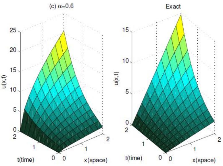
Fig. 6. 3D Graphical representation of solution (4.13) of IVP (4.8)-(4.9) when a = 0.6 and exact solution (4.14) with respect to time

Loading Preview
Sorry, preview is currently unavailable. You can download the paper by clicking the button above.
References (40)
- Kilbas AA, et al. Theory and applications of fractional differential equations. Elsevier, Amsterdam, The Netherlands; 2016.
- Oldham KB, Spanier J. The fractional calculus. Academic Press, New York, NY, USA; 1974.
- Caputo M, Mainardi F. Linear models of dissipation in anelastic solids. Rivista Del Nuovo Cimento. 1971;1(2):161-198.
- Duan JS, et al. A review of decomposition method and its application to fractional differential equations. Comm. in Fractional Calculus. 2012;3(2):73-99.
- Mainardi Carpinteri F. Fractals and fractional calculus in continuum mechanics. Springer Verlag, Wien and New York. 1997;223-276.
- Magin RL. Fractional Calculus in Bio-engineering. Begell House Publisher, Inc., Connecticut; 2006.
- Miller KS, Ross B. An introduction to the fractional calculus and fractional differential equations. Wiley, New York; 1993.
- Duan JS, Rach R. Higher-order numeric WazwazEl-Sayed modified Adomian decomposition algorithms. Computers and Mathematics with Applications. 2012;63(11):1557-1568.
- Khodabakhshi N, et al. Numerical solutions of the initial value problem for fractional differential equations by modification of the Adomian decomposition method. Fractional Calculus and Applied Analysis. 2014;17(2):82-400.
- Lu T, Zheng Q. Adomian decomposition method for first order PDEs with unprescribed data. Alexandria Engineering Journal. 2021;60(2):2563-2572.
- Sobamowo GM, et al. Application of Adomian decomposition method to free vibration analysis of thin isotropic rectangular plates submerged in fluid. Journal of the Egyptian Mathematical Society. 2020;28(1):1-17.
- Srivastava HM, et al. A new analysis of the time-fractional and space-time fractional-order Nagumo equation. Journal of Informatics and Mathematical Sciences. 2018;10(4):545-561.
- Adomain G. Solving frontier problems of physics: The Decomposition Method, Kluwer, Boston; 1994.
- Adomain G. A review of decomposition method in applied mathematics. J. Math. Anl. Appl. 1988;135:501-544.
- Wazwaz AM. Partial differential equations. Methods and Applications, Balkema Publishers, Leiden, The Netherlands; 2002.
- Wazwaz AM. The decomposition method applied to systems of partial differential equations and to the reaction-diffusion Brusselator model. Appl. Math. Comput. 2000;110:251-264.
- Shawagfeh NT. Analytical approximate solution for nonlinear fractional differential equations. Appl. Math. Comput. 2000;131(2):517-529.
- Jafari H, Daftardar-Gejji V. Solving linear and nonlinear fractional diffusion and wave equations by Adomian decomposition. Appl. Math. Comput. 2006;180(2):488-497.
- Jafari H, Daftardar-Gejji V. Adomian decomposition: a tool for solving a system of fractional differential equations. J. Math. Anal. Appl. 2005;301(2):508-518.
- Dhaigude DB, et al. Adomian decomposition method for fractional Benjamin-Bona-Mahony- Burgers equations. Int. J. Appl. Math. Mech. 2012;8(12):4251.
- Dhaigude DB, Birajdar GA. Numerical solution of system of fractional partial differ ential equations by discrete Adomian decomposition method. J. Frac. Cal. Appl. 2012;3(12):1-11.
- Chitalkar-Dhaigude C, Bhadgaonkar V. Adomian Decomposition Method Over Charpits Method for Solving Nonlinear First Order Partial Differential Equations. Bull. Marathwada Math. Soc. 2017;18(1):118.
- Dhaigude DB, Bhadgaonkar VN. Analytical solution of nonlinear nonhomogeneous space and time fractional physical models by improved Adomian decomposition method. Punjab University Journal of Mathematics; 2021. In press.
- Sontakke BR, Pandit R. Convergence analysis and approximate solution of fractional differential equations. Malaya Journal of Matematik (MJM). 2019;7(2):338-344.
- Sontakke BR. Adomian decomposition method for solving highly nonlinear fractional partial diffeential equations. IOSR journal of Engineering (IOSRJEN). 2019;9(3):39-44.
- Sontakke BR, Pandit R. Numerical solution of time fractional time regularized long wave equation by Adomian decomposition method and applications. Journal of Mechanics of Continua and Mathematical Sciences. 2021;16(2):48-60.
- Guo P. The Adomian decomposition method for a type of fractional differential equations. J. Appl. Math. Phys. 2019;7:2459-2466.
- Biazar J, Eslami M. Differential transform method for nonlinear fractional gas dynamics equation. Inter. J. Phys. Sci. 2011;6(5):1203-1206.
- Das, S. and Kumar, R. (2011). Approximate analytical solutions of fractional gas dynamics.Appl. Math. Comput., 217(24),9905-9915.
- Kumar S, Rashidi MM. New analytical method for gas dynamics equation arising in shock fronts. Comput. Phys. Commun. 2014;185(7):19471954.
- Hajmohammadi MR, et al. Semianalytical treatments of conjugate heat transfer. J. Mech. Eng. Sci. 2012;227(3): 492503.
- Tamsir M, Shrivastava VK. Revisiting the approximate analytical solution of fractional-order gas dynamics equation. Alexandria Engineering Journal. 2016;55(2):867-874.
- Hahn DW, Ozisik MN. Heat conduction, Wiley; 2012.
- Narasimhan TN. Fouriers heat conduction equation: History, influences and connections. Proc. Indian Acad. Sci. 1999;108(3):117148.
- Fakour M, et al. Analytical study of micropolar fluid flow and heat transfer in a channel with permeable walls. Journal of Molecular Liquids. 2015;204:198-204.
- Fakour M, et al. Scrutiny of underdeveloped nanofluid MHD flow and heat conduction in a channel with porous walls. International Journal of Case Studies in Thermal Engineering. 2014;4:202-214.
- Fakour M, et al. Study of heat transfer in nanofluid MHD flow in a channel with permeable walls. begellhouse, Heat Transfer Research. 2017;48(3):221-238.
- Fakour M, et al. Study of heat transfer and flow of nanofluide in permeable channel in the presence of magnetic field. Propulsion and Power Research. 2015;4(1):50-62.
- Fakour M, et al. Nanofluide thin film flow and heat transfer over an unsteady stretching elastic sheet by LSM. Journal of Mechanical Science and Technology. 2018;32(1):177-183.
- Rahbari A, et al. Heat transfer and fluid flow of blood with nanoparticles through porous vessels in a magnetic field: A quasi-one dimensional analytical approach. Mathematical Biosciences. 2017;283:38-47.