Investigation of Dynamic Characteristics of Multi-Bladed S-Shaped Vane Type Rotor (original) (raw)
2014, Journal of Mechanical Engineering
Abstract
In the present research work the dynamic conditions of Multi S-shaped bladed rotor at different Reynolds number have been identified. The investigation on wind loading and aerodynamic effects on the four, five and six bladed S-shaped vertical axis vane type rotor has been conducted with the help of an open circuit subsonic wind tunnel. For different bladed rotor the flow velocities were varied from 5m/s to 9m/s covering the Reynolds numbers up to 1.35 x 10⁵. It was experiential that by increasing the number of blades of rotor to the optimum limit considering all significant factors and at the same time by increasing its Reynolds number, the power output can be increased to its maximum level Finally, the nature of predicted dynamic characteristics has been examined by comparing with the existing research works. DOI: http://dx.doi.org/10.3329/jme.v44i1.19501
Figures (134)
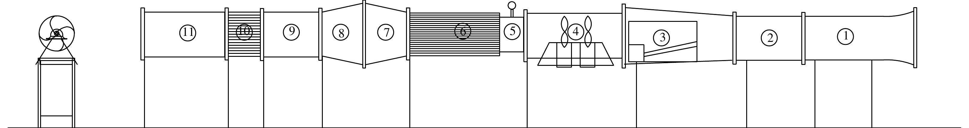

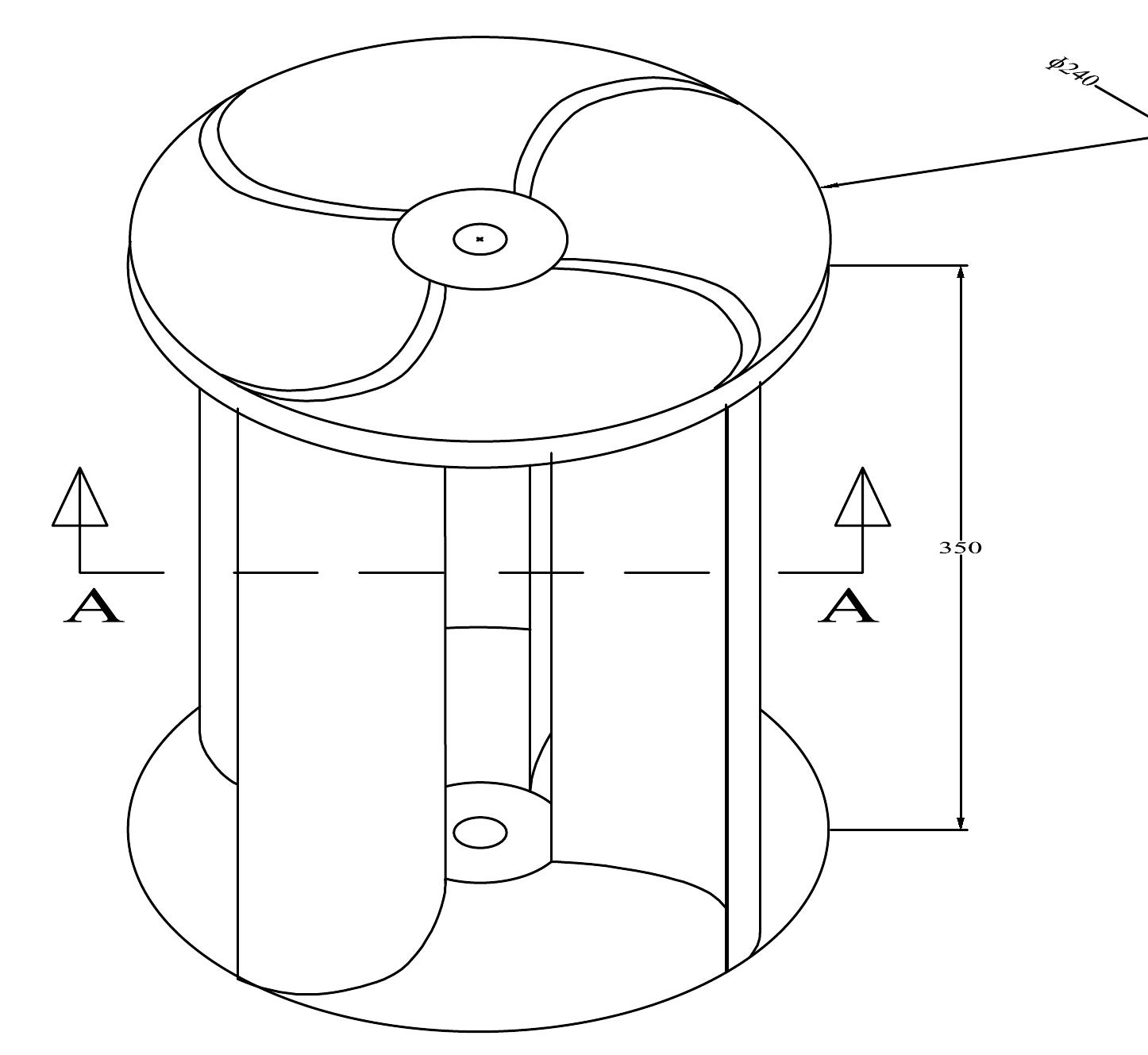


Figure 5.4.3 (b): Three Dimensional View of Five Bladed Vertical Axis Vane Type Rotor


Wind energy is an indirect form of solar energy. The sun radiates 1014 kJ/sec of energy to the earth. Sufficient amount of energy is continuously transferred from the sun to the air of earth. Some of the sun’s energy is absorbed directly by air. Most of the energy of the sun is first absorbed by the surface of the earth and then transferred to air by convection. Between 1-2% of the solar radiation that reaches the earth is converted into wind energy. Global wind pattern depends mainly on the earth’s rotation around its own axis, ocean current and cosmic gravitational pulls. However, the prime cause of local wind is different. The Earth is unevenly heated by the sun, such that the poles receive less energy from the sun than the equator; along with this, dry land heats up (and cools down) more quickly than the seas do. Cold air over the sea then replaces the rising air. The diagram below shows how this ‘system’ works. The differential heating drives a global atmospheric convection system reaching from the Earth's surface to the stratosphere which acts as a virtual ceiling. Most of the energy stored in these wind movements can be found at high altitudes where continuous wind speeds of over 160 km/h (99 mph) occur. Eventually, the wind energy is converted through friction into diffuse heat throughout the Earth's surface and the atmosphere.

Vertical-axis windmills were also used in China, which is often claimed as _ their birthplace. While the belief that the windmill was invented in China more than 2000 years ago is widespread and may be accurate, the earliest actual documentation of a Chinese windmill was in 1219 A.D. by the Chinese statesman Yehlu Chhu-Tshai. Here also, the primary applications were apparently grain grinding and water pumping.

Figure 2.2.2: The Brush windmill (the first use of a large windmill to generate electricity.) in Cleveland, Ohio, 1888. sy the 14th century, Dutch windmills were in use to drain areas of the Rhine River delta n Denmark by 1900, there were about 2500 windmills for mechanical loads such a: umps and mills, producing an estimated combined peak power of about 30 MW. The irst known electricity generating windmill operated was a battery charging machine nstalled in 1887 by James Blyth in Scotland. The first windmill for electricity productior n the United States was built in Cleveland, Ohio by Charles F Brush in 1888 (Figure .2.2), and in 1908 there were 72 wind-driven electric generators from 5 kW to 25 kW ‘he largest machines were on 24 m (79 ft) towers with four-bladed 23 m (75 ft) diameter: otors. Around the time of World War I, American windmill makers were producing 00,000 farm windmills each year, mostly for water-pumping. By the 1930s, windmills or electricity were common on farms, mostly in the United States where distributior ystems had not yet been installed. In this period, high-tensile steel was cheap, anc vindmills were placed a top prefabricated open steel lattice towers. A forerunner of modern horizontal-axis wind generators was in service at Yalta, USSR in 1931. This was a 100 kW generator on a 30 m (100 ft) tower, connected to the local 6.3 kV distribution system. It was reported to have an annual capacity factor of 32 per cent, not much different from current wind machines. In the fall of 1941, the first megawatt- class wind turbine was synchronized to a utility grid in Vermont. The Smith-Putnam wind turbine only ran for 1100 hours. Due to war time material shortages the unit was not repaired.
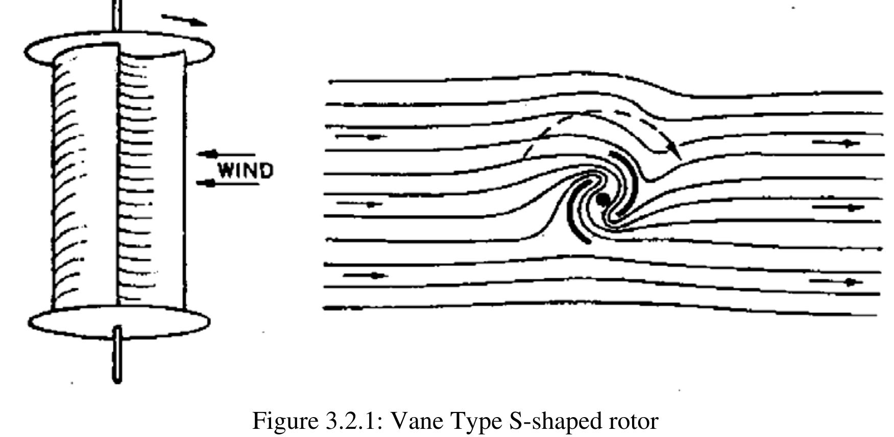
The Vane type rotor of S-shaped cross section (fig. 3.2.1) 1s predominantly drag based. but also uses a certain amount of aerodynamic lift. Drag based vertical axis wind turbines have relatively higher starting torque and less rotational speed than their lift based counterparts. Furthermore, their power output to weight ratio is also less. Because of the low speed, these are generally considered unsuitable for producing electricity, although 11 is possible by selecting proper gear trains. Drag based windmills are useful for other applications such as grinding grain, pumping water and a small output of electricity. A major advantage of drag based vertical axis wind turbines lies in their self—starting capacity, unlike the Darrieus lift—based vertical axis wind turbines. but also uses a certain amount of aerodynamic lift. Drag based vertical axis wind turbines
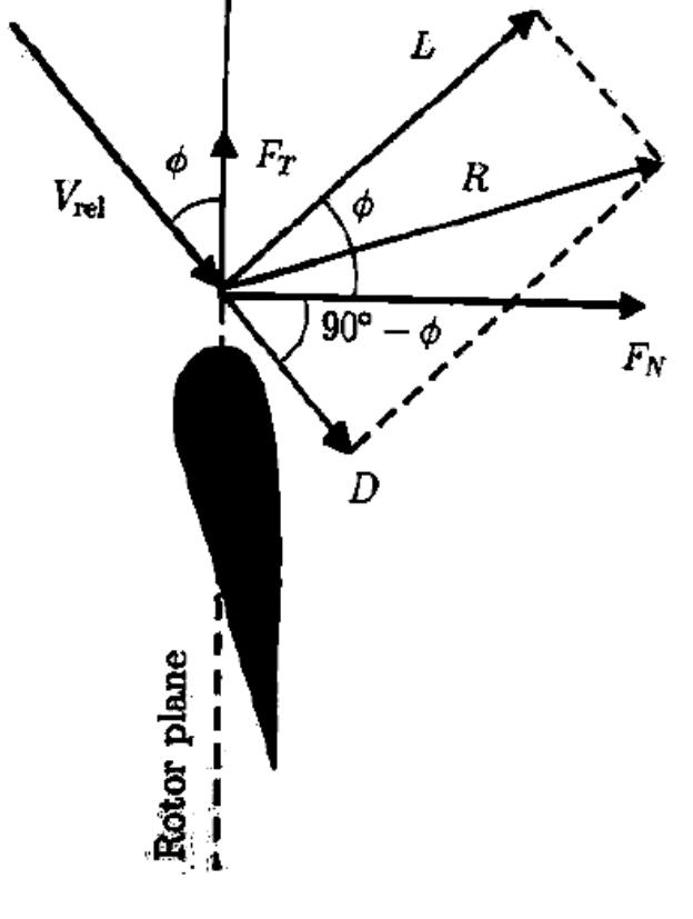
perpendicular and parallel to the relative wind as shown The lift and drag coefficient values are usually obtained experimentally and correlated against the Reynolds number. A section of a blade at radius r is illustrated in Fig. 3.4.1, with the associated velocities, forces and angles shown. The relative wind vector at radius r, is denoted by V,.;, and the angle of the relative wind speed to the plane of rotation, by . The resultant lift and drag forces are represented by L and D, which are directly perpendicular and parallel to the relative wind as shown A careful choice of the rotor blades geometry and shape modification is crucial for maximum efficiency. Wind turbines have typically used airfoils based on the wings of airplanes, although new airfoils are specially designed for use on rotors. Airfoils use the concept of lift, as opposed to drag, to harness the wind’s energy. Blades that operate with lift (forces perpendicular to the direction of flow) are more efficient than a drag machine. Certain curved and rounded shapes have resulted most efficient in employing lift. When the edge of the airfoil is angled slightly out of the direction of the wind, the air moves
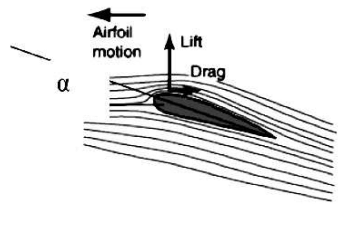
operating conditions with a low blade angle of attack, a, thus favors the lift force. Bernoulli’s principle indicates how faster flow implies lower pressure on the airfoil:
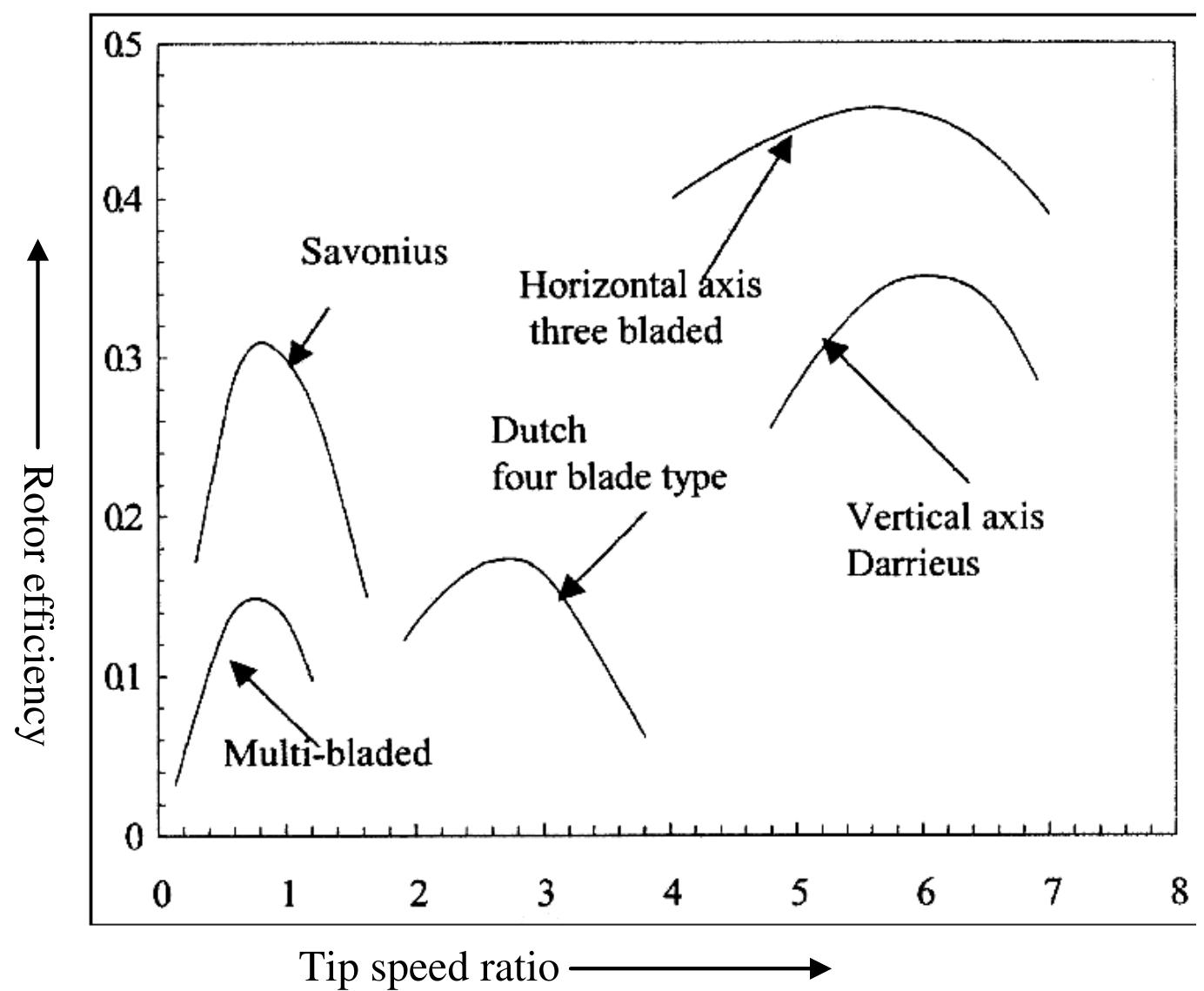
![Figure 3.4.3: Rotor efficiency vs. downstream / upstream wind speed ratio [35] As with all turbines, only a part of the energy shown in fig. 3.4.4 can be extracted. If too much kinetic energy were removed, the exiting air flow would stagnate and thus cause blockage. When the air flow approaches the inlet of the turbine, it meets a blockage imposed by the rotor-stator blades. This causes a decrease in kinetic energy, while the static pressure increases to a maximum at the turbine blade. As the air continues through the turbine, energy in the fluid is transferred to the turbine rotor blades, while the static pressure drops below the atmospheric pressure as fluid flows away from the rotor. This will eventually further reduce the kinetic energy. Then kinetic energy from the surrounding wind is entrained to bring it back to the original state.](https://figures.academia-assets.com/96774948/figure_014.jpg) ](
](Figure 3.4.3: Rotor efficiency vs. downstream / upstream wind speed ratio [35] As with all turbines, only a part of the energy shown in fig. 3.4.4 can be extracted. If too much kinetic energy were removed, the exiting air flow would stagnate and thus cause blockage. When the air flow approaches the inlet of the turbine, it meets a blockage imposed by the rotor-stator blades. This causes a decrease in kinetic energy, while the static pressure increases to a maximum at the turbine blade. As the air continues through the turbine, energy in the fluid is transferred to the turbine rotor blades, while the static pressure drops below the atmospheric pressure as fluid flows away from the rotor. This will eventually further reduce the kinetic energy. Then kinetic energy from the surrounding wind is entrained to bring it back to the original state.

Typical velocity and pressure distributions are illustrated in Figure 3.4.4, using the disk actuator model and Betz limit theory. If the stream tube model is applied to a vertical axis wind turbine, it gives insight into the velocity and pressure distributions for a multi- bladed S-shaped vane type wind turbine. Because of the continuity principle for the stream tube, the diameter of the flow field must experience an increase as the velocity decreases giving rise to a sudden pressure drop, { p'=(p" —p,;)}, at the rotor plane. This pressure drop contributes to the torque for rotating turbine blades. wind turbine, it gives insight into the velocity and pressure distributions for a multi- bladed S-shaped vane type wind turbine. Because of the continuity principle for the
![Figure 3.6.1: Plan view of actuator cylinder to analyze vertical axis wind turbines [41] The multiple-streamtube model is a well established technique for predicting the performance of vertical axis wind turbines. It is similar in many ways to that used fot horizontal axis wind turbines. The objective of the analysis is to simultaneously determine the forces acting on the blades of the turbine by a “blade element analysis” and deceleration of the wind that occurs due to the energy extracted from the air flow by the turbine, through actuator strip theory. As the rotor of the vertical axis wind turbine revolves, the blades trace the path of a vertical cylinder known as the actuator cylinder. As the wind intersects this cylinder, it must slow and any given streamtube of rectangulat cross section must expand horizontally as shown schematically in Figure 3.6.1. cross section must expand horizontally as shown schematically in Figure 3.6.1.](https://figures.academia-assets.com/96774948/figure_017.jpg) ](
](Figure 3.6.1: Plan view of actuator cylinder to analyze vertical axis wind turbines [41] The multiple-streamtube model is a well established technique for predicting the performance of vertical axis wind turbines. It is similar in many ways to that used fot horizontal axis wind turbines. The objective of the analysis is to simultaneously determine the forces acting on the blades of the turbine by a “blade element analysis” and deceleration of the wind that occurs due to the energy extracted from the air flow by the turbine, through actuator strip theory. As the rotor of the vertical axis wind turbine revolves, the blades trace the path of a vertical cylinder known as the actuator cylinder. As the wind intersects this cylinder, it must slow and any given streamtube of rectangulat cross section must expand horizontally as shown schematically in Figure 3.6.1. cross section must expand horizontally as shown schematically in Figure 3.6.1.
![Figure 3.6.2: Lift and drag force on vertical axis wind turbine [41]](https://figures.academia-assets.com/96774948/figure_018.jpg) ](
](Figure 3.6.2: Lift and drag force on vertical axis wind turbine [41]
![Figure 3.6.3: Velocities at the rotor plane [34] Figure 3.6.4: Schematic of blade elements](https://figures.academia-assets.com/96774948/figure_019.jpg) ](
](Figure 3.6.3: Velocities at the rotor plane [34] Figure 3.6.4: Schematic of blade elements
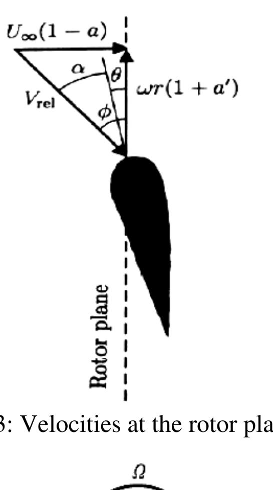

Figures 3.6.2 and 3.6.3 show that lift and drag forces, L and D, respectively, could be determined and hence the torque, power output from the blades and mechanical efficiency of the rotor could be determined. Here the symbol £ represents the blade azimuth angle, @ is the angle between the resultant wind velocity, V, and the blade velocity (wr), a is the angle of attack, y is the blade pitch angle and 0 is the angle between the streamtube and the rotor radius. The relative wind velocity V;e1, (W) is the vector sum of the wind velocity at the rotor U. (1— a) (vector sum of the free-stream wind velocity, V.o and the induced axial velocity - aV..) and the wind velocity due to rotation of the blade. The rotational component is the sum of the velocity due to the blades motion, (@r), and the swirl velocity of the air, a' (@r) . The axial velocity U.» (1- a), is reduced by a component U.. a, due to the wake effect or retardation imposed by the blades, where Ux is the upstream undisturbed wind speed. The relative wind velocity is shown on the velocity diagram in Figure 3.6.3. The minus sign in the term Us (1- a) is due to retardation of flow as the air comes into contact with the rotor. The positive sign in the term o.r(1+ a’ ) occurs due to the flow of air in the reverse direction of blade rotation, after air particles contact the blades and yields torque. This flow ahead and behind the rotor is not completely axial, as assumed in an ideal case. When the air exerts torque to the rotor, as a reaction, a rotational wake is generated behind the rotor. Depending on the wake length or separation, an energy loss is experienced, which resulted in a reduction of the power coefficient. efficiency of the rotor could be determined. Here the symbol B represents the blade


Figure 5.4.1: Constructional Details of the Test Section
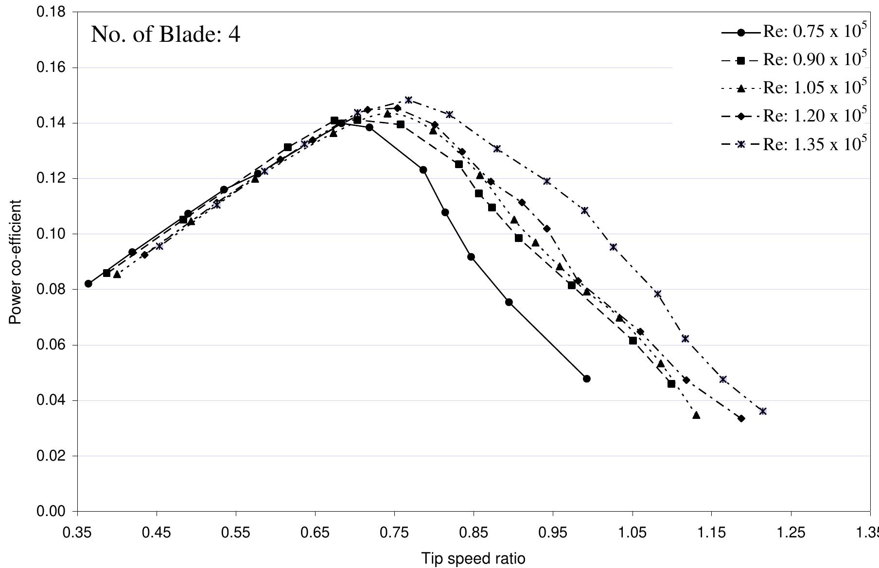
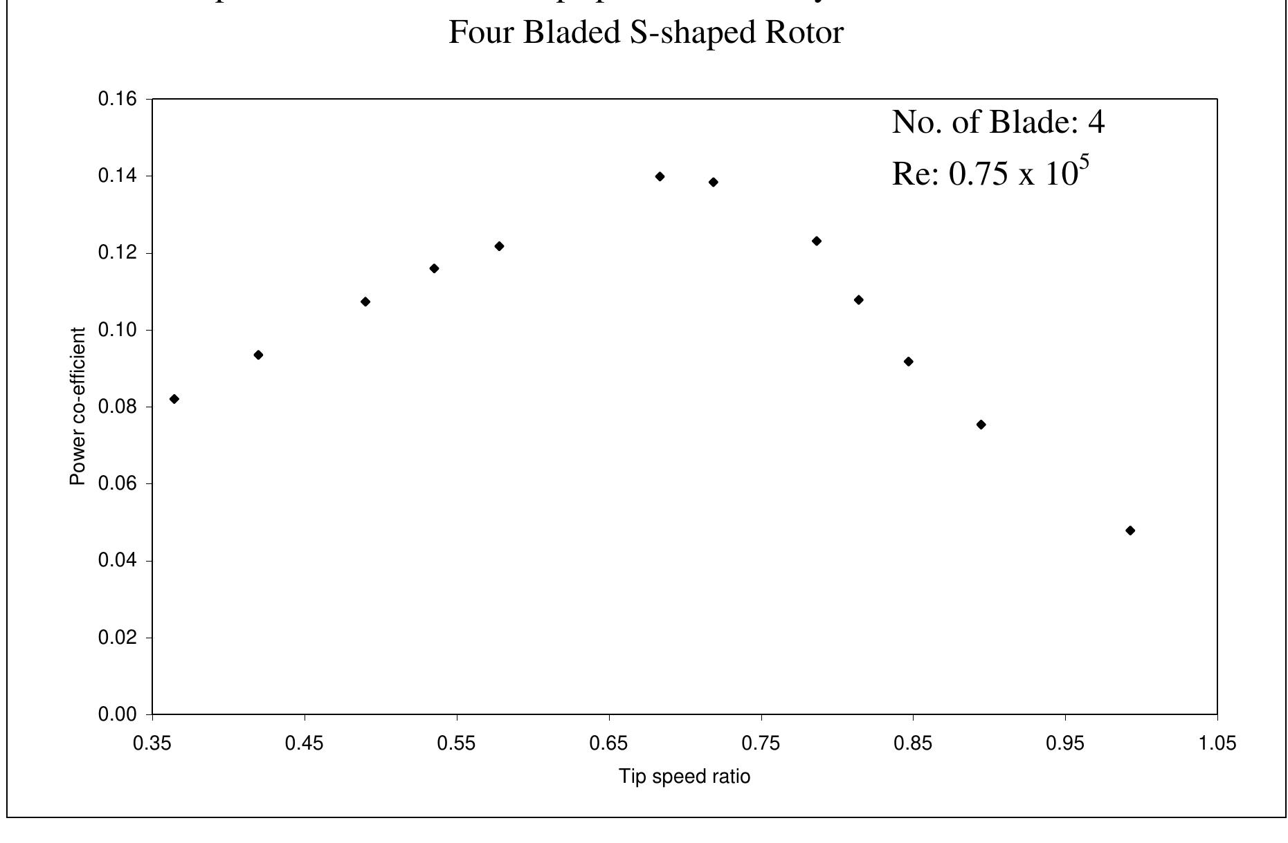
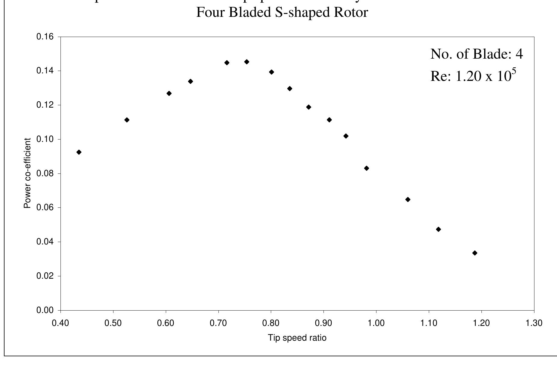
nature of power co-efficient versus tip speed ratio curve slightly steeper. From this graph it is evident that with the increase of Reynolds number the maximum value of power coefficient also increases and it is shifted towards the higher values of tip speed ratios. So, it can be concluded that the increase of Reynolds number make the nature of power co-efficient versus tip speed ratio curve slightly steeper. Figure 6.2.1: Comparisons of power coefficient vs. tip speed ratio for Four Bladed S- shaped Rotor at different Reynolds number

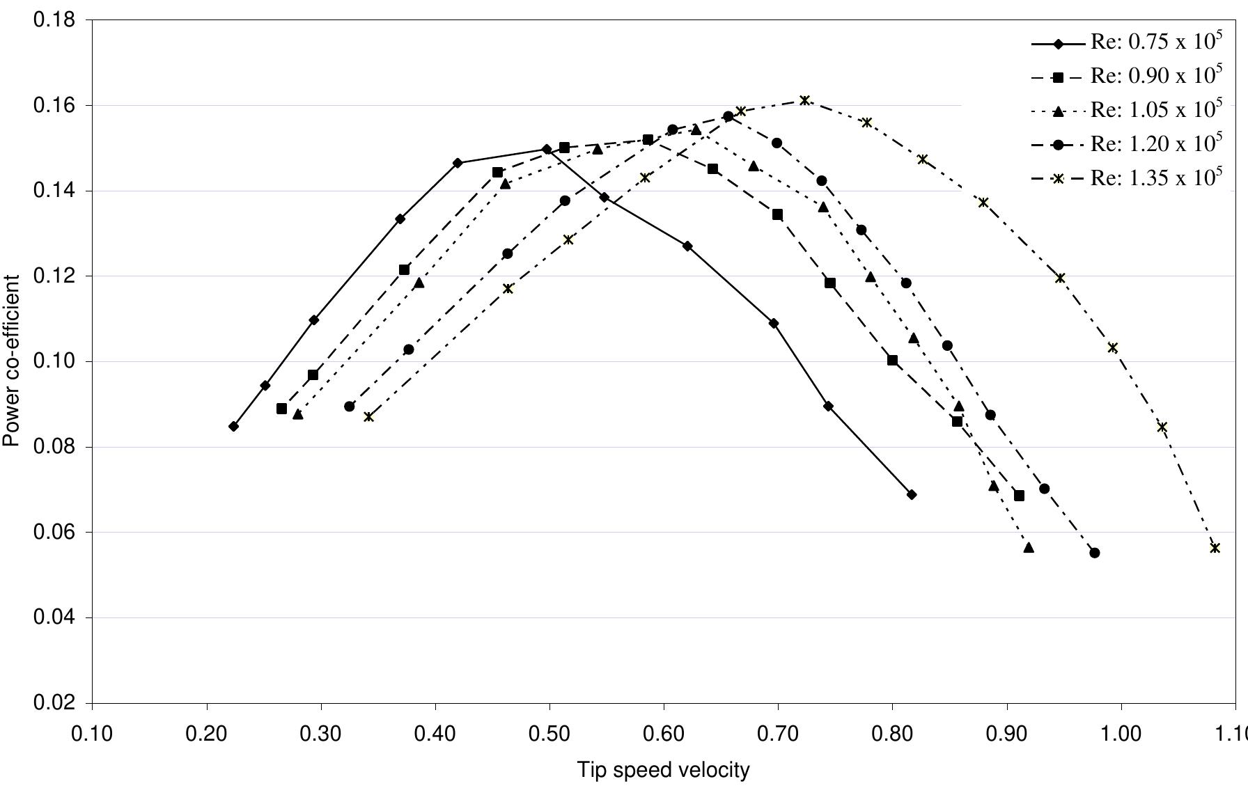
Figure 6.2.2: Comparisons of power coefficient vs. tip speed ratio for Five Bladed S- shaped Rotor at different Reynolds number nature of power co-efficient versus tip speed ratio curve slightly sharper.

) speed ratio as the number of blades in the same sized rotor is increased. Figure 6.2.4: Comparisons of power coefficient versus tip speed ratio of 4, 5 and 6 bladed rotors at Reynolds number of 0.75 x 10°
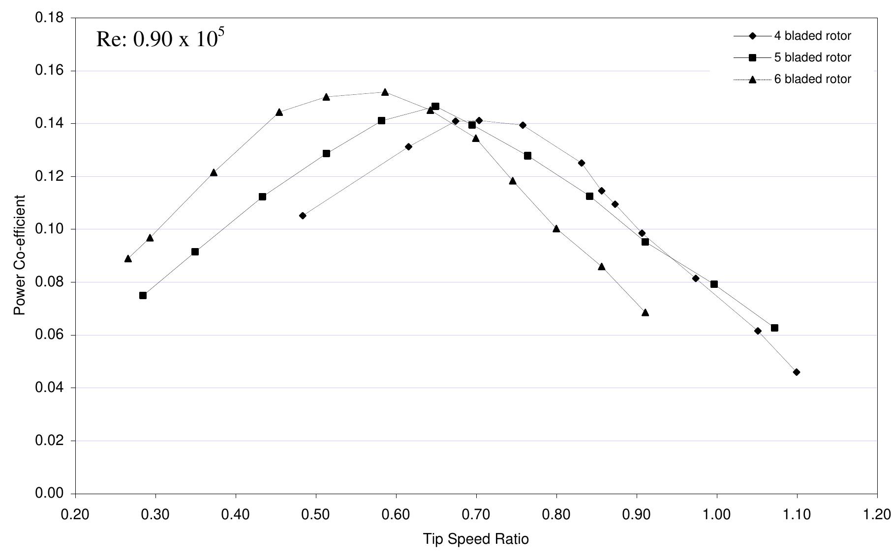

Figure 6.2.6: Comparisons of power coefficient versus tip speed ratio of 4, 5 and 6 bladed rotors at Reynolds number of 1.05 x 10°
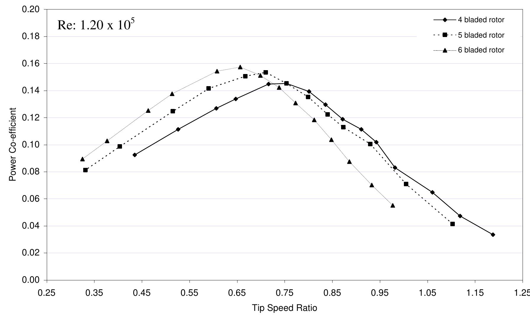

Figure 6.2.8: Comparisons of power coefficient versus tip speed ratio of 4, 5 and 6 bladed rotors at Reynolds number of 1.35 x 10°

Figure 6.2.9: Comparisons of torque coefficient versus tip speed ratio for Four Bladed S- shaped Rotor at different Reynolds number

Figure 6.2.10: Comparisons of torque coefficient versus tip speed ratio for Five Bladed S-shaped Rotor at different Reynolds number

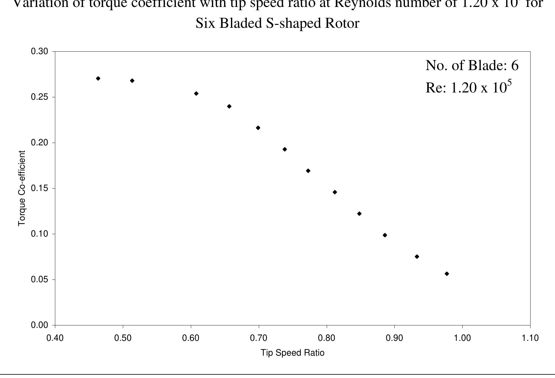
Figure 6.2.11: Comparisons of torque coefficient versus tip speed ratio for Six Bladed S-shaped Rotor at different Reynolds number

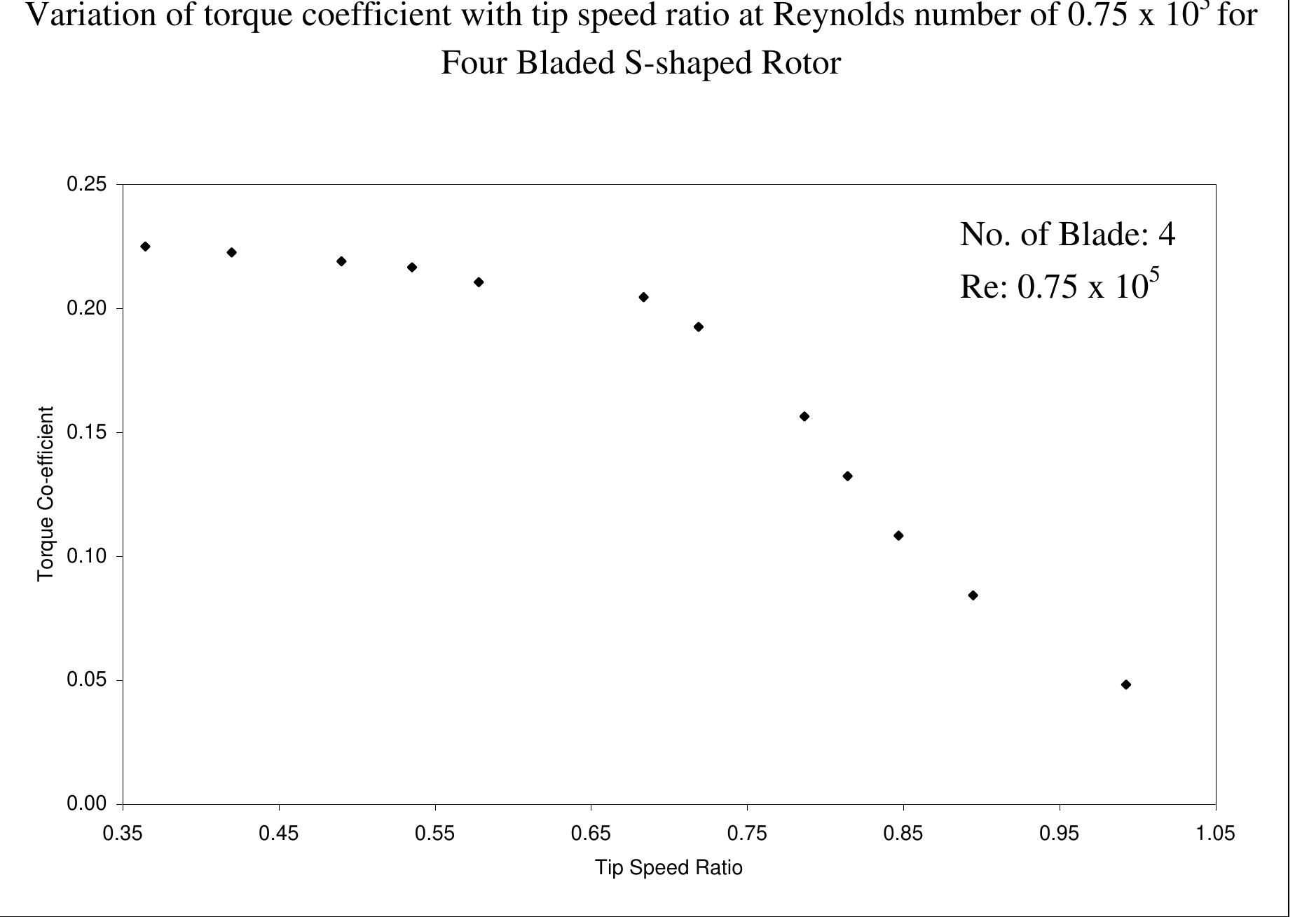
Figure 6.2.12: Comparisons of torque coefficient versus tip speed ratio of 4, 5 and 6 bladed rotors at Reynolds number of 0.75 x 10° speed ratio as the number of blades in the same sized rotor is increased. In Figures 6.2.13 to 6.2.16 the same thing can be observed. For 4, 5 and 6 bladed rotors a Reynolds number of 0.90 x 10° maximum torque coefficients of 0.2214, 0.2631 anc 0.3342 occur at tip speed ratios of 0.3875, 0.2848 and 0.2660 respectively. Similarly, a Reynolds number of 1.05 x 10°, 1.20 x 10° and 1.35 x 10° it can be observed that th value of maximum torque co-efficient becomes higher for higher number of bladed roto and this maximum value of torque co-efficient is shifted towards the lower value of ti speed ratio as the number of blades in the same sized rotor is increased.


Figure 6.2.14: Comparisons of torque coefficient versus tip speed ratio of 4, 5 and 6 bladed rotors at Reynolds number of 1.05 x 10°


Figure 6.2.16: Comparisons of torque coefficient versus tip speed ratio of 4, 5 and 6 bladed rotors at Reynolds number of 1.35 x 10°

![Figure 6.2.18: Comparisons of torque coefficient versus tip speed ratio of present and existing experimental results [28]](https://figures.academia-assets.com/96774948/figure_042.jpg) ](
](Figure 6.2.18: Comparisons of torque coefficient versus tip speed ratio of present and existing experimental results [28]

![Figure 6.2.20: Comparisons of torque coefficient versus tip speed ratio of present and existing experimental results [28]](https://figures.academia-assets.com/96774948/figure_044.jpg) ](
](Figure 6.2.20: Comparisons of torque coefficient versus tip speed ratio of present and existing experimental results [28]

![Figure 6.2.22: Comparisons of torque coefficient versus tip speed ratio of present and existing experimental results [5, 21]](https://figures.academia-assets.com/96774948/figure_046.jpg) ](
](Figure 6.2.22: Comparisons of torque coefficient versus tip speed ratio of present and existing experimental results [5, 21]

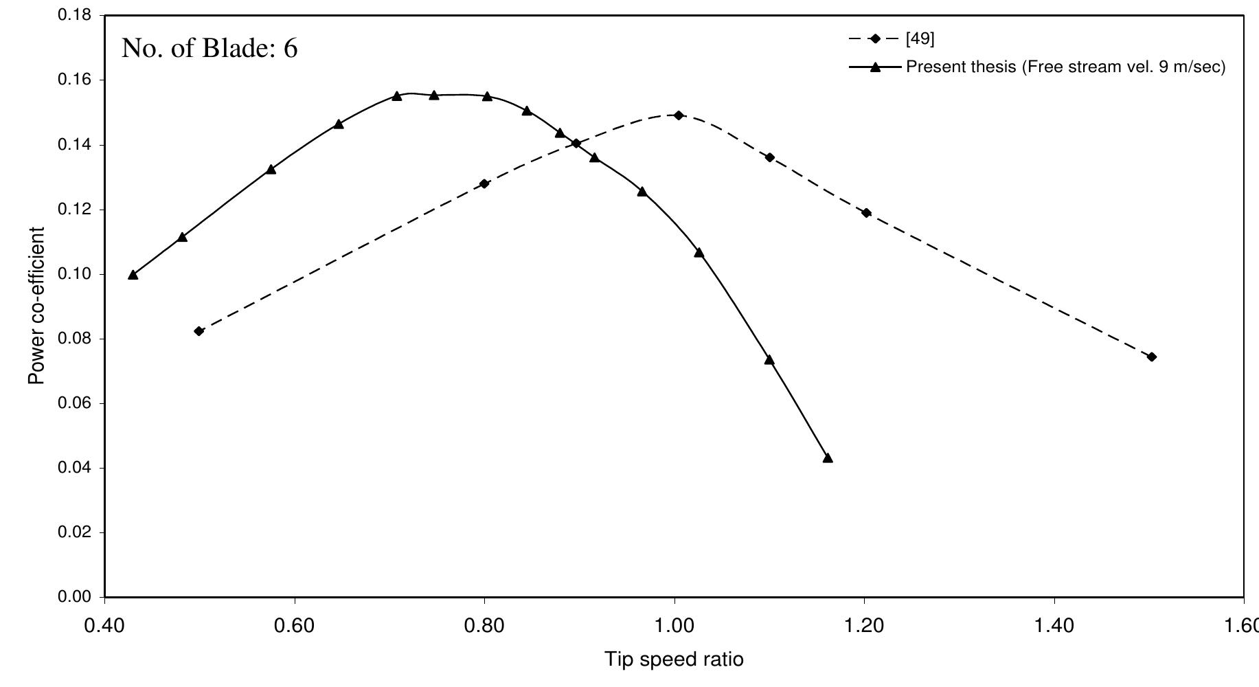
![Figure 6.2.24: Comparisons of torque coefficient versus tip speed ratio of present and existing experimental results [49] for four bladed rotor](https://figures.academia-assets.com/96774948/figure_048.jpg) ](
](Figure 6.2.24: Comparisons of torque coefficient versus tip speed ratio of present and existing experimental results [49] for four bladed rotor


![Figure 6.2.30: Comparisons of torque coefficient versus tip speed ratio of present and existing experimental results [17]](https://figures.academia-assets.com/96774948/figure_054.jpg) ](
](Figure 6.2.30: Comparisons of torque coefficient versus tip speed ratio of present and existing experimental results [17]
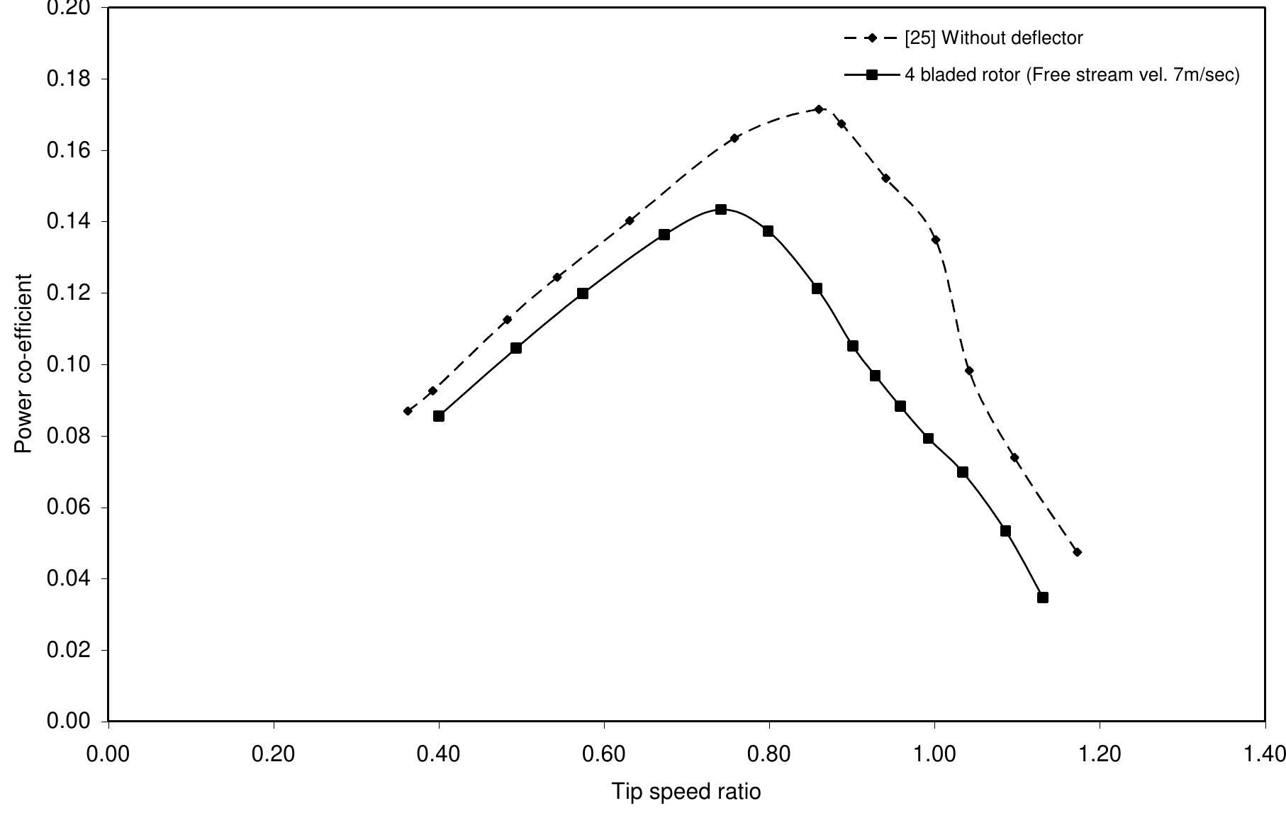
![Figure 6.2.32: Comparisons of torque coefficient versus tip speed ratio of present and existing experimental results [25]](https://figures.academia-assets.com/96774948/figure_056.jpg) ](
](Figure 6.2.32: Comparisons of torque coefficient versus tip speed ratio of present and existing experimental results [25]

Table 5.2.1: Performance of Savonius/ S-shaped rotor


These squat structures, typically (at least) four bladed, usually with wooden shutters or fabric sails, were developed in Europe. These windmills were pointed into the wind manually or via a tail-fan and were typically used to grind grain. In the Netherlands they were also used to pump water from low-lying land, and were instrumental in keeping its polders dry.

Horizontal axis disadvantages
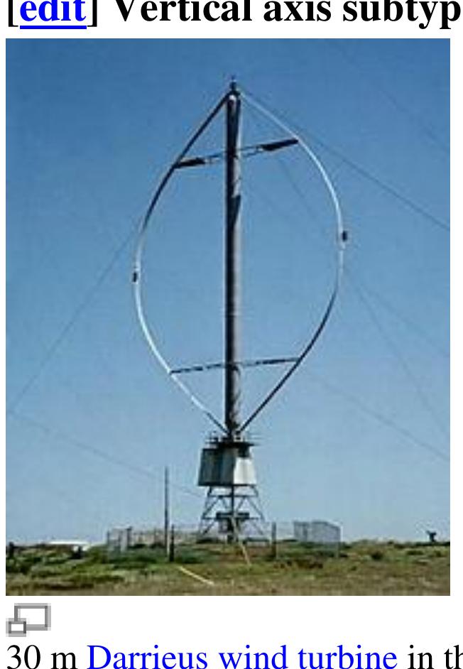
"Eggbeater" turbines, or Darrieus turbines, were named after the French inventor, Georges Darrieus."”! They have good efficiency, but produce large torque ripple and cyclical stress on the tower, which contributes to poor reliability. They also generally require some external power source, or an additional Savonius rotor to start turning, because the starting torque is very low. The torque ripple is reduced by using three or more blades which results in a higher solidity for the rotor. Solidity is measured by blade area divided by the rotor area. Newer Darrieus type turbines are not held up by guy-wires but have an external superstructure connected to the top bearing.
ratio which lowers blade bending stresses. Straight, V, or curved blades may be used.

![Monthly average wind speeds in the island [IFRD, 2002] Wind Data From Bangladesh Meteorological Department_in Bangladesh: Available wind speeds in the Saint Martin’s Island are presented in the Table 3.7 below.](https://figures.academia-assets.com/96774948/table_018.jpg) ](
](Monthly average wind speeds in the island [IFRD, 2002] Wind Data From Bangladesh Meteorological Department_in Bangladesh: Available wind speeds in the Saint Martin’s Island are presented in the Table 3.7 below.

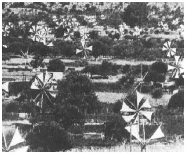
Figure 2. Water Pumping Sailwing Machines on the Island of Crete

Figure 3. An early sail-wing horizontal-axis mill on the Mediterranean coast Windmills in the Western World (1300 - 1875 A.D.)

In 1891, the Dane Poul La Cour developed the first electrical output wind machine to incorporate the aerodynamic design principles (low-solidity, four-bladed rotors incorporating primitive airfoil shapes) used in the best European tower mills. The higher speed of the La Cour rotor made these mills quite practical for electricity generation. By the close of World War I, the use of 25 kilowatt electrical output machines had spread throughout Denmark, but cheaper and larger fossil-fuel steam plants soon put the operators of these mills out of business.

Figure 7. M.L. Jacobs adjusting the spring-actuated pitch change mechanism on a Jacobs Wind- electric in 1977.

Figure 8. Palmer Putnam's 1.25-megawatt wind turbine was one of the engineering marvels of th late 1930's, but the jump in scale was too great for available materials.

Figure 9. Yes, that's an airframe holding together the three blades of the "Gedser Mollen." Fiberglass later eliminated this design requirement.

These squat structures, typically (at least) four bladed, usually with wooden shutters or fabric sails, were developed in Europe. These windmills were pointed into the wind manually or via a tail-fan and were typically used to grind grain. In the Netherlands they were also used to pump water from low-lying land, and were instrumental in keeping its polders dry.


"Eggbeater" turbines, or Darrieus turbines, were named after the French inventor, Georges Darrieus."“” They have good efficiency, but produce large torque ripple and cyclical stress on the tower, which contributes to poor reliability. They also generally require some external power source, or an additional Savonius rotor to start turning, because the starting torque is very low. The torque ripple is reduced by using three or more blades which results in a higher solidity for the rotor. Solidity is measured by blade area divided by the rotor area. Newer Darrieus type turbines are not held up by guy-wires but have an external superstructure connected to the top bearing.

ratio which lowers blade bending stresses. Straight, V, or curved blades may be used.


To begin to understand the complex physics involved in wind turbine aerodynamics, < simple one-dimensional model should be analyzed. In the one-dimensional Rankine Froude actuator disc model, the rotor is represented by an “actuator disc,” through whick the static pressure has a jump discontinuity. Let us consider a control volume fixed i1 space whose external boundaries are the surface of a stream tube whose fluid passe: through the rotor disc, a cross-section of the stream tube upwind of the rotor, and a cross. section of the stream tube downwind of the rotor. This theory is useful in the derivatiot of ideal efficiency of a rotor of wind turbines. A simple schematic of this control volume is given in Fig. 3.1.

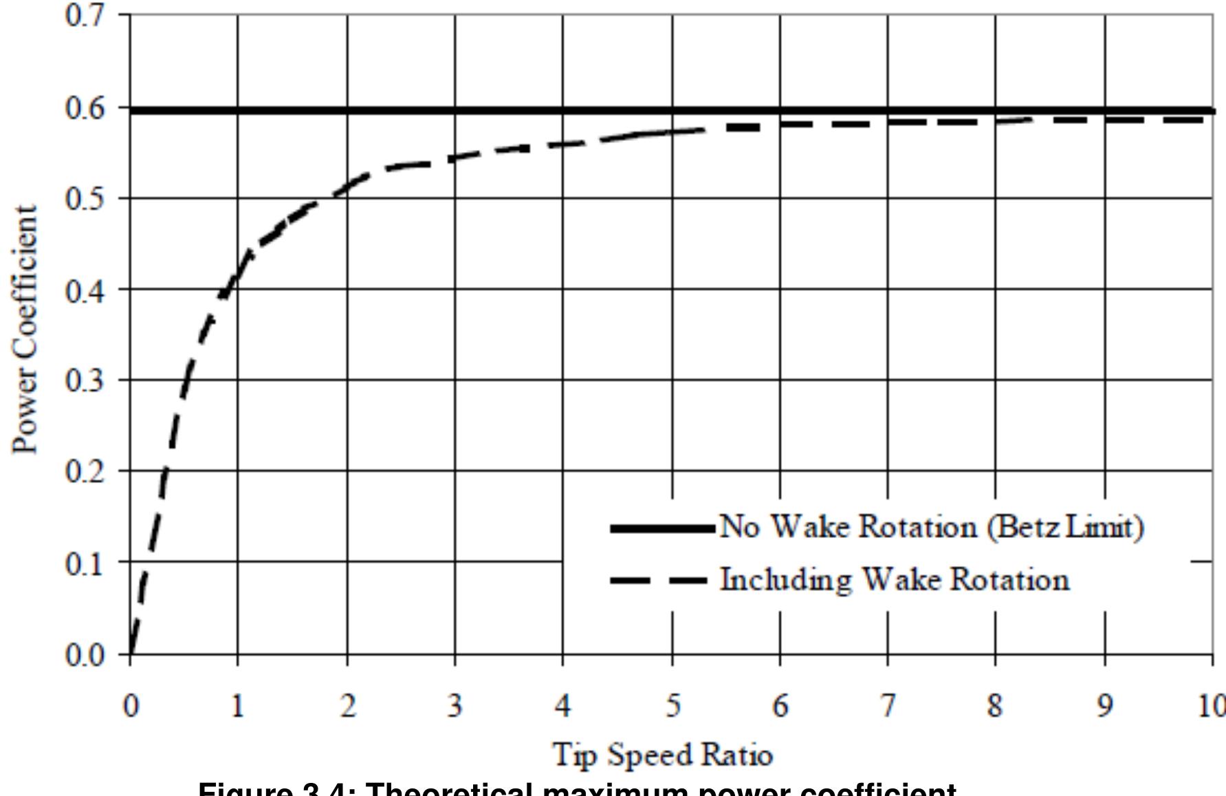
Figure 3.2: Stream Tube Model showing the Rotation of Wake Since the wake is now rotating, it exhibits rotational kinetic energy that reduces the amount of available energy that can be extracted as useful work. As explained in the subsequent analysis, a rotor generating high torque at low speed will generate less power than a rotor generating low torque at high speed. The typical multi-bladed farm windmill is a notable example of a wind turbine whose efficiency is severely limited by wake rotation. subsequent analysis, a rotor generating high torque at low speed will generate less power In the previous model, assumption (1) stated that the rotor imparted no angular momentum to the wake. However, conserving angular momentum necessitates rotation of the wake if the rotor is to extract useful torque. Moreover, the flow behind the rotor will rotate in the opposite direction as the rotor in reaction to the flow imparting torque on the rotor as shown in Fig. 3.2. is a notable example of a wind turbine whose efficiency is severely limited by wake

Figure 3.3: Annular stream tube control volumes power to all functions of the annular radius. This point of view is illustrated in Fig. 3.3: local pressures, axial velocities (and induction factor), angular velocities, thrust, and Assumption (3) in the analysis of the Rankine-Froude actuator disc model could have been relaxed in the analysis if the variables Ai, T, and P were replaced with the differentials, dA;, dT, and dP, respectively. In this case, the differential area of an annular ring at station i, dAj, is defined as:
Strip theory Solidity affects Grit affects on airfoil performance Stalling and furling

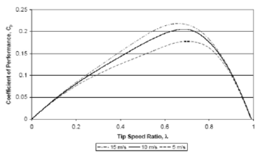
Figure 8. Performance of the Wollongong Turbine predicted for three wind speeds, assuming blade lift and drag data can be approximated by that for NACA0012H (Whitten, 2002). The analysis carried out by Whitten (2002) must be viewed as preliminary for a number o feasons, including the fact that lift and drag data were not available for the symmetric blade profile used in practice. As a starting point Whitten used lift and drag data for the NACADO12F blade (Sheldahl and Klimas, 1981) and interpolated for both angle of attack and Reynolds number. Other limitations of his analysis include the fact that no tip losses were included.

Loading Preview
Sorry, preview is currently unavailable. You can download the paper by clicking the button above.
References (53)
- Templin, R.J., -Aerodynamic Performance Theory for the NRC Vertical-Axis Wind Turbine‖, National Research Council of Canada, Report LTR-LA-160, June 1974.
- Wilson, R.E. and Lissaman, P.B.S., -Applied Aerodynamics of Wind Power Machines‖, Oregon State University, 1974.
- Park, J. -Simplified Wind Power System for Experimenters‖ , Helion Inc., California, USA, 1975.
- Strickland, J.H., -The Darrieus Turbine: A Performance Prediction Model using Multiple Streamtubes, Sandia Laboratories Report‖, SAND75-0431, 1975.
- Littler, R.D., -Further Theoretical and Experimental Investigation of the Savonius Rotor‖, B.E. Thesis, University of Queensland, 1975.
- Swamy, N.V.C. and Fritzsche, A.A., -Aerodynamic Studies on Vertical Axis Wind Turbine‖, International Symposium on Wind Energy Systems, Cambridge, England, September 7-9, 1976.
- Fanucci, J.B. and Watters, R.E., -Innovative Wind Machines: The Theoretical Performance of a Vertical-Axis Wind Turbine‖, Proceedings of the Vertical-Axis Wind Turbine Technology Workshop, Sandia Laboratories, SAND 76-5586, P.P. III-61-95, 1976.
- Holme, O., -A Contribution to the Aerodynamic Theory of the Vertical Axis Wind Turbine‖, Proceedings of the International Symposium on Wind Energy Systems, Cambridge, p.p. C4-55-72, 1976.
- Jansen, W.A.M. and Smulders, P.T., -Rotor Design for Horizontal Axis Windmills‖, Steering Committee for Wind Energy in Developing Countries (SWD), P.O. Box 85, Amersfoort, The Netherlands, 1977.
- Sheldahi, R.E., Blackwell, B.F. and Feltz, L.V., -Wind Tunnel Performance Data for Two and Three Bucket Savonius Rotors‖, Journal of Energy, vol.2, No.3, 1977.
- Lysen, E.H., Bos, H.G. and Cordes, E.H., -Savonius Rotors for Water Pumping‖, SWD publication, P.O. Box 85, Amersfoort, The Netherlands, 1978.
- Beurskens, H.J.M., -Feasibility Study of Windmills for Water Supply in Mara Region, Tanzania‖, Steering Committee on Wind Energy for Developing Countries (SWD), P.O. Box 85, Amersfoort, The Netherlands, 1978.
- Alexander, A.J. and B.P. Holownia, -Wind Tunnel Tests on a Savonius Rotor‖, J. Industrial Aerodynamics, vol. 3, 1978.
- Beurskens, H.J.M., -Low Speed Water Pumping Wind Mills: Rotor Tests and Overall Performance‖' Proc. of 3 rd Int. Symp. On Wind Energy Systems, Copenhagen, Denmark, August 26-29, pp K2 501-520, 1980.
- Noll, R.B. and Ham, N.D., -Analytical Evaluation of the Aerodynamic Performance of a Hi-Reliability Vertical-Axis Wind Turbine‖, Proceedings of AWEA National Conference, 1980.
- Baird, J.P. and Pender, S.F., -Optimization of a Vertical Axis Wind Turbine for Small Scale Applications, 7 th Australian Hydraulic and Fluid Mechanics Conference, Brisbane, 1980.
- Bergeles, G. and Athanassiadis N., -On the Flow Field of the Savonius Rotor‖, Journal of Wind Engineering, vol. 6, 1982.
- Lysen, E.H., -Introduction to Wind Energy‖, 2 nd Edition, SWD Publication, P.O. Box 85, Amersfoort, The Netherlands, 1983.
- Paraschivoiu, I. and Delclaux, F., -Double Multiple Stream Tube Model with Recent Improvements‖, Journal of Energy, vol. 7, no. 3, p.p. 250-255, 1983.
- Sivasegaram, S. and Sivapalan, S., -Augmentation of Power in Slow Running Vertical Axis Wind Rotors using Multiple Vanes‖, Journal of Wind Engineering, vol. 7, no. 1, 1983.
- Bowden, G.J. and McAleese, S.A., -The Properties of Isolated and Coupled Savonius Rotors‖, Journal of Wind Engineering, vol. 8, no. 4, pp. 271-288, 1984.
- Paraschiviu, I., Fraunic, P. and Beguier, C., -Stream Tube Expansion Effects on the Darrieus Wind Turbine‖, Journal of Propulsion, vol. 1, no. 2, pp. 150-155, 1985.
- Mandal, A.C., -Aerodynamics and Design Analysis of Vertical Axis Darrieus Wind Turbine‖, Ph.D. Thesis Vrije University Brussel, Belgium 1986.
- Sawada, T., Nakamura, M. and Kamada, S., -Blade Force Measurement and Flow Visualization of Savonius Rotors‖, Bull. JSME. Vol.29, pp. 2095-2100, 1986.
- Ogawa, T. and Yoshida, H., -The Effects of a Deflecting Plate and Rotor End Plates‖, Bulletin of JSME, vol. 29, no. 253, pp. 2115-2121, 1986.
- Aldos, T.K. and Obeidat, K.M., -Performance Analysis of Two Savonius Rotors Running Side by Side Using The Discrete Vortex Method‖, Wind Engineering, Vol. 11, No. 5, 1987.
- Gavalda, J., Massons, J. and Diaz, F., -Drag and Lift Coefficients of the Savonius Wind Machine‖, Wind Engineering, Vol. 15, pp. 240-246, 1991.
- Huda, M.D., Selim, M.A., Islam, A.K.M.S. and Islam, M.Q., -The Perfomance of an S-Shaped Savonius Rotor with a Deflecting Plate‖ RERIC International Energy Journal: Vol. 14, No. 1, pp. 25-32, June 1992.
- Islam, A.K.M.S., Islam, M.Q., Mandal, A.C. and Razzaque, M.M. -Aerodynamic Characteristics of a Stationary Savonius Rotor‖, RERIC Int. Energy Journal, Vol. 15, No. 2, pp. 125-135, 1993.
- Islam, A.K.M.S., Islam, M.Q., Razzaque, M.M. and Ashraf, R., -Static Torque and Drag Characteristics of an S-Shaped Savonius Rotor and Prediction of Dynamic Characteristics‖, Wind Engineering, Vol. 19, No. 6, U.K., 1995.
- Burton, J.D., Hijazin, M. and Rizvi, S., -Wind and Solar Driven Reciprocating Lift Pumps‖, Journal of Wind Engineering. Vol.15, No. 2: pp 95-108, 1995.
- Fujisawa, N., -Velocity Measurements and Numerical Calculations of Flow Fields in and around Savonius Rotors‖ Journal of Wind Engineering and Industrial Aerodynamics, Vol. 59, Issue 1, Pages 39-50, January 1996.
- Rasmussen, F., Petersen, J.T., Volund, P., Leconte, P., Szechenyi, E., Westergaard, C., -Soft Rotor Design for Flexible Turbines‖ Research funded in part by THE EUROPEAN COMMISSION in the framework of the Non Nuclear Energy Programme JOULE 3.EC, 1998.
- Spera, D. A., -Wind Turbine Technology‖, ASME Press, 1998
- Patel, M.R., Wind and Solar Power Systems, CRC Press, NY, 1999.
- Rahman, M., -Aerodynamic Characteristics of a Three Bladed Savonius Rotor‖, M.Sc. Engg. Thesis, Dept of Mechanical Engg., BUET, 2000.
- Ammara, I., Leclerc, L., and Masson, C., -A Viscous Three Dimensional Differential/ Actuator-Disk Method for the Aerodynamic Analysis of Wind Farms,‖ Journal of Solar Energy Engineering, vol. 124, pp. 345 -356, November, 2002.
- Bhuiyan, H. K, -Aerodynamic Characteristics of a Four Bladed Savonius Rotor‖, M.Sc. Engg. Thesis, Dept of Mech. Engg., BUET, 2003.
- Iida, A., Mizuno, A. and Fukudome, K., -Numerical Simulation of Aerodynamic Noise Radiated form Vertical Axis Wind Turbines‖, Proceedings of the 18 International Congress on Acoustics, 2004.
- Hyosung, S. and Soogab, L. -Response Surface Approach to Aerodynamic Optimization Design of Helicopter Rotor Blade‖ Vol. 64, no. 1, pp. 125-142 [18 page(s) (article)] (19 ref.), 2005.
- Cooper P. and Kennedy O., -Development and Analysis of a Novel Vertical Axis Wind Turbine‖ University of Wollongong, Wollongong, 3, 2005.
- Song, S.H., Jeong, B.C., Lee, H.I., J.J., Oh, J.H. and Venkataramanan, G., -Emulation of Output Characteristics of Rotor Blades using a Hardware -in-loop Wind Turbine Simulator‖ Volume 3, Issue, Page(s): 1791-1796, 6-10 March 2005.
- Saha, U.K. and Rajkumar, M.J., -On the performance analysis of Savonius rotor with twisted blades‖ Department of Mechanical Engineering, Indian Institute of Technology Guwahati, Guwahati-781 039, August 2005.
- Islam, M.Q., Hasan, M.N. and Saha, S., -Experimental Investigation of Aerodynamic Characteristics of Two, Three and Four Bladed S-Shaped Stationary Savonius Rotors‖ Proceedings of the International Conference on Mechanical Engineering (ICME05-FL-23), Dhaka-1000, Bangladesh, 28-30 December 2005.
- Maeda, T. and Kawabuchi, H., -Effect of Wind Shear on the Characteristics of a Rotating Blade of a Field Horizontal Axis Wind Turbine‖ Journal of Fluid Science and Technology, Vol. 2, No. 1 pp. 152-162, 2007.
- Gupta, R., Biswas, A. and Sharma K.K., -Comparative study of a three-bucket Savonius rotor with a combined three-bucket Savonius-three-bladed Darrieus rotor‖ Department of Mechanical Engineering, National Institute of Technology (NIT), Silchar 788 010, Assam, India, December 2007.
- Saha, U.K. and Maity, D., -Optimum Design Configuration of Savonius Rotor through Wind Tunnel Experiments‖, Journal of Wind Engineering and Industrial Aerodynamics, Volume 96, Issues 8-9, Pages 1359-1375, August-September 2008.
- Ajedegba, J.O., -Effects of Blade Configuration on Flow Distribution and Power Output of a Zephyr Vertical Axis Wind Turbine‖, M.Sc. Engg. Thesis, Dept of Mech. Engg., The Faculty of Engineering and Applied Science, University of Ontario Institute of Technology, July, 2008.
- Kamal, F.M. and Islam, M.Q., -Aerodynamic Characteristics of a Stationary Five Bladed Vertical Axis Vane Type Wind Turbine‖ Journal of Mechanical Engineering, Vol. ME39, No. 2, IEB, December 2008.
- Wind Speeds in the Saint Martin's Island : Available wind speeds in the Saint Martin's Island are presented in the Table 3.7 below. Monthly average wind speeds in the island [IFRD, 2002]
- Month V av (m/s) V max (m/s)
- is again the static pressure at station i. Pressures p 0 and p 3 are identical by assumption (4), so pressures p 1 and p 2 can be eliminated from the thrust Eq. (3.4.4) with the help of Eqs. (3.4.5) to obtain: (3.4.6) Eliminating thrust at the rotor disc from Eqs. (3.4.3) and (3.4.6), the velocity of the flow through the rotor disc is the average of the upwind (free stream) and downwind velocities: (3.4.
- An axial induction (or interference) factor, a, is customarily defined as the fractional decrease in wind velocity between the free stream and the rotor plane: (3.4.22) by virtue of Eq. (3.4.17). The ½ is used in the definition of the angular induction factor a' since the angular velocity of the flow stream at the plane of the rotor (at the jump discontinuity), ω, the average value of the angular velocity just upwind and downwind of the rotor: (3.4.23) or: and (3.4.