Comprehensive Guide to Text Summarization using Deep Learning in Python (original) (raw)

Introduction

“I don’t want a full report, just give me a summary of the results”. I have often found myself in this situation – both in college as well as my professional life. We prepare a comprehensive report and the teacher/supervisor only has time to read the summary.

Sounds familiar? Well, I decided to do something about it. Manually converting the report to a summarized version is too time taking, right? Could I lean on Natural Language Processing (NLP) techniques to help me out?

This is where the awesome concept of Text Summarization using Deep Learning really helped me out. It solves the one issue which kept bothering me before – now our model can understand the context of the entire text. It’s a dream come true for all of us who need to come up with a quick summary of a document!

And the results we achieve using text summarization in deep learning? Remarkable. So in this article, we will walk through a step-by-step process for building a Text Summarizer using Deep Learning by covering all the concepts required to build it. And then we will implement our first text summarization model in Python!

Note: This article requires a basic understanding of a few deep learning concepts. I recommend going through the below articles.

• A Must-Read Introduction to Sequence Modelling (with use cases)
• Must-Read Tutorial to Learn Sequence Modeling (deeplearning.ai Course #5)
• Essentials of Deep Learning: Introduction to Long Short Term Memory

Table of contents

• Introduction
• What is Text Summarization in NLP?
  • Extractive Summarization
  • Abstractive Summarization
• Introduction to Sequence-to-Sequence (Seq2Seq) Modeling
• Understanding the Encoder-Decoder Architecture
  • Training phase
  • Inference Phase
• Limitations of the Encoder – Decoder Architecture
• The Intuition behind the Attention Mechanism
  • Global Attention
  • Local Attention
• Understanding the Problem Statement
• Implementing Text Summarization in Python using Keras
  • Custom Attention Layer
  • Import the Libraries
  • Read the dataset
  • Drop Duplicates and NA values
  • Preprocessing
  • a) Text Cleaning
  • b) Summary Cleaning
  • Understanding the distribution of the sequences
  • Preparing the Tokenizer
  • Model building
  • Understanding the Diagnostic plot
• How can we Improve the Model’s Performance Even Further?
• How does the Attention Mechanism Work?
• Conclusion
• Frequently Asked Questions

I’ve kept the ‘how does the attention mechanism work?’ section at the bottom of this article. It’s a math-heavy section and is not mandatory to understand how the Python code works. However, I encourage you to go through it because it will give you a solid idea of this awesome NLP concept.

What is Text Summarization in NLP?

Let’s first understand what text summarization is before we look at how it works. Here is a succinct definition to get us started:

“Automatic text summarization is the task of producing a concise and fluent summary while preserving key information content and overall meaning”

-Text Summarization Techniques: A Brief Survey, 2017

Text summarization refers to the technique of condensing a lengthy text document into a succinct and well-written summary that captures the essential information and main ideas of the original text, achieved by highlighting the significant points of the document.

There are broadly two different approaches that are used for text summarization:

• Extractive Summarization
• Abstractive Summarization

Let’s look at these two types in a bit more detail.

The name gives away what this approach does. We identify the important sentences or phrases from the original text and extract only those from the text. Those extracted sentences would be our summary. The below diagram illustrates extractive summarization:

I recommend going through the below article for building an extractive text summarizer using the TextRank algorithm:

• An Introduction to Text Summarization using the TextRank Algorithm (with Python implementation)

Abstractive Summarization

This is a very interesting approach. Here, we generate new sentences from the original text. This is in contrast to the extractive approach we saw earlier where we used only the sentences that were present. The sentences generated through abstractive summarization might not be present in the original text:

You might have guessed it – we are going to build an Abstractive Text Summarizer using Deep Learning in this article! Let’s first understand the concepts necessary for building a Text Summarizer model before diving into the implementation part.

Exciting times ahead!

Introduction to Sequence-to-Sequence (Seq2Seq) Modeling

We can build a Seq2Seq model on any problem which involves sequential information. This includes Sentiment classification, Neural Machine Translation, and Named Entity Recognition – some very common applications of sequential information.

In the case of Neural Machine Translation, the input is a text in one language and the output is also a text in another language:

In the Named Entity Recognition, the input is a sequence of words and the output is a sequence of tags for every word in the input sequence:

Our objective is to build a text summarizer where the input is a long sequence of words (in a text body), and the output is a short summary (which is a sequence as well). So, we can model this as a Many-to-Many Seq2Seq problem. Below is a typical Seq2Seq model architecture:

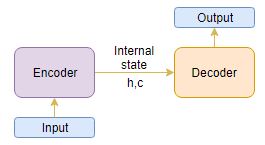
There are two major components of a Seq2Seq model:

• Encoder
• Decoder

Let’s understand these two in detail. These are essential to understand how text summarization works underneath the code. You can also check out this tutorial to understand sequence-to-sequence modeling in more detail.

Understanding the Encoder-Decoder Architecture

The Encoder-Decoder architecture is mainly used to solve the sequence-to-sequence (Seq2Seq) problems where the input and output sequences are of different lengths.

Let’s understand this from the perspective of text summarization. The input is a long sequence of words and the output will be a short version of the input sequence.

Generally, variants of Recurrent Neural Networks (RNNs), i.e. Gated Recurrent Neural Network (GRU) or Long Short Term Memory (LSTM), are preferred as the encoder and decoder components. This is because they are capable of capturing long term dependencies by overcoming the problem of vanishing gradient.

We can set up the Encoder-Decoder in 2 phases:

• Training phase
• Inference phase

Let’s understand these concepts through the lens of an LSTM model.

Training phase

In the training phase, we will first set up the encoder and decoder. We will then train the model to predict the target sequence offset by one timestep. Let us see in detail on how to set up the encoder and decoder.

Encoder

An Encoder Long Short Term Memory model (LSTM) reads the entire input sequence wherein, at each timestep, one word is fed into the encoder. It then processes the information at every timestep and captures the contextual information present in the input sequence.

I’ve put together the below diagram which illustrates this process:

The hidden state (hi) and cell state (ci) of the last time step are used to initialize the decoder. Remember, this is because the encoder and decoder are two different sets of the LSTM architecture.

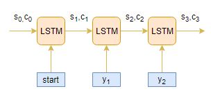
Decoder

The decoder is also an LSTM network which reads the entire target sequence word-by-word and predicts the same sequence offset by one timestep. The decoder is trained to predict the next word in the sequence given the previous word.

and <end> are the special tokens which are added to the target sequence before feeding it into the decoder. The target sequence is unknown while decoding the test sequence. So, we start predicting the target sequence by passing the first word into the decoder which would be always the <start> token. And the <end> token signals the end of the sentence.

Pretty intuitive so far.

Inference Phase

After training, the model is tested on new source sequences for which the target sequence is unknown. So, we need to set up the inference architecture to decode a test sequence:

How does the inference process work?

Here are the steps to decode the test sequence:

1. Encode the entire input sequence and initialize the decoder with internal states of the encoder
2. Pass <start> token as an input to the decoder
3. Run the decoder for one timestep with the internal states
4. The output will be the probability for the next word. The word with the maximum probability will be selected
5. Pass the sampled word as an input to the decoder in the next timestep and update the internal states with the current time step
6. Repeat steps 3 – 5 until we generate <end> token or hit the maximum length of the target sequence

Let’s take an example where the test sequence is given by [x1, x2, x3, x4]. How will the inference process work for this test sequence? I want you to think about it before you look at my thoughts below.

1. Encode the test sequence into internal state vectors
2. Observe how the decoder predicts the target sequence at each timestep:

Time step: t=1

Time step: t=2

And, Time step: t=3

Limitations of the Encoder – Decoder Architecture

As useful as this encoder-decoder architecture is, there are certain limitations that come with it.

• The encoder converts the entire input sequence into a fixed length vector and then the decoder predicts the output sequence. This works only for short sequences since the decoder is looking at the entire input sequence for the prediction
• Here comes the problem with long sequences. It is difficult for the encoder to memorize long sequences into a fixed length vector

“A potential issue with this encoder-decoder approach is that a neural network needs to be able to compress all the necessary information of a source sentence into a fixed-length vector. This may make it difficult for the neural network to cope with long sentences. The performance of a basic encoder-decoder deteriorates rapidly as the length of an input sentence increases.”

-Neural Machine Translation by Jointly Learning to Align and Translate

So how do we overcome this problem of long sequences? This is where the concept of attention mechanism comes into the picture. It aims to predict a word by looking at a few specific parts of the sequence only, rather than the entire sequence. It really is as awesome as it sounds!

The Intuition behind the Attention Mechanism

How much attention do we need to pay to every word in the input sequence for generating a word at timestep t? That’s the key intuition behind this attention mechanism concept.

Let’s consider a simple example to understand how Attention Mechanism works:

• Source sequence: “Which sport do you like the most?
• Target sequence: “I love cricket”

The first word ‘I’ in the target sequence is connected to the fourth word ‘you’ in the source sequence, right? Similarly, the second-word ‘love’ in the target sequence is associated with the fifth word ‘like’ in the source sequence.

So, instead of looking at all the words in the source sequence, we can increase the importance of specific parts of the source sequence that result in the target sequence. This is the basic idea behind the attention mechanism.

There are 2 different classes of attention mechanism depending on the way the attended context vector is derived:

• Global Attention
• Local Attention

Let’s briefly touch on these classes.

Global Attention

Here, the attention is placed on all the source positions. In other words, all the hidden states of the encoder are considered for deriving the attended context vector:

Source: Effective Approaches to Attention-based Neural Machine Translation – 2015

Local Attention

Here, the attention is placed on only a few source positions. Only a few hidden states of the encoder are considered for deriving the attended context vector:

Source: Effective Approaches to Attention-based Neural Machine Translation – 2015

We will be using the Global Attention mechanism in this article.

Understanding the Problem Statement

Customer reviews can often be long and descriptive. Analyzing these reviews manually, as you can imagine, is really time-consuming. This is where the brilliance of Natural Language Processing can be applied to generate a summary for long reviews.

We will be working on a really cool dataset. Our objective here is to generate a summary for the Amazon Fine Food reviews using the abstraction-based approach we learned about above.

You can download the dataset from here.

Implementing Text Summarization in Python using Keras

It’s time to fire up our Jupyter notebooks! Let’s dive into the implementation details right away.

Custom Attention Layer

Keras does not officially support attention layer. So, we can either implement our own attention layer or use a third-party implementation. We will go with the latter option for this article. You can download the attention layer from here and copy it in a different file called attention.py.

Let’s import it into our environment:

Import the Libraries

Read the dataset

This dataset consists of reviews of fine foods from Amazon. The data spans a period of more than 10 years, including all ~500,000 reviews up to October 2012. These reviews include product and user information, ratings, plain text review, and summary. It also includes reviews from all other Amazon categories.

We’ll take a sample of 100,000 reviews to reduce the training time of our model. Feel free to use the entire dataset for training your model if your machine has that kind of computational power.

Drop Duplicates and NA values

Preprocessing

Performing basic preprocessing steps is very important before we get to the model building part. Using messy and uncleaned text data is a potentially disastrous move. So in this step, we will drop all the unwanted symbols, characters, etc. from the text that do not affect the objective of our problem.

Here is the dictionary that we will use for expanding the contractions:

We need to define two different functions for preprocessing the reviews and generating the summary since the preprocessing steps involved in text and summary differ slightly.

a) Text Cleaning

Let’s look at the first 10 reviews in our dataset to get an idea of the text preprocessing steps:

data['Text'][:10]

Output:

We will perform the below preprocessing tasks for our data:

• Convert everything to lowercase
• Remove HTML tags
• Contraction mapping
• Remove (‘s)
• Remove any text inside the parenthesis ( )
• Eliminate punctuations and special characters
• Remove stopwords
• Remove short words

Let’s define the function:

b) Summary Cleaning

And now we’ll look at the first 10 rows of the reviews to an idea of the preprocessing steps for the summary column:

Output:

Define the function for this task:

Remember to add the START and END special tokens at the beginning and end of the summary:

Now, let’s take a look at the top 5 reviews and their summary:

Output:

Understanding the distribution of the sequences

Here, we will analyze the length of the reviews and the summary to get an overall idea about the distribution of length of the text. This will help us fix the maximum length of the sequence:

Output:

Interesting. We can fix the maximum length of the reviews to 80 since that seems to be the majority review length. Similarly, we can set the maximum summary length to 10:

We are getting closer to the model building part. Before that, we need to split our dataset into a training and validation set. We’ll use 90% of the dataset as the training data and evaluate the performance on the remaining 10% (holdout set):

Preparing the Tokenizer

A tokenizer builds the vocabulary and converts a word sequence to an integer sequence. Go ahead and build tokenizers for text and summary:

a) Text Tokenizer

b) Summary Tokenizer

Model building

We are finally at the model building part. But before we do that, we need to familiarize ourselves with a few terms which are required prior to building the model.

• Return Sequences = True: When the return sequences parameter is set to True, LSTM produces the hidden state and cell state for every timestep
• Return State = True: When return state = True, LSTM produces the hidden state and cell state of the last timestep only
• Initial State: This is used to initialize the internal states of the LSTM for the first timestep
• Stacked LSTM: Stacked LSTM has multiple layers of LSTM stacked on top of each other. This leads to a better representation of the sequence. I encourage you to experiment with the multiple layers of the LSTM stacked on top of each other (it’s a great way to learn this)

Here, we are building a 3 stacked LSTM for the encoder:

Output:

I am using sparse categorical cross-entropy as the loss function since it converts the integer sequence to a one-hot vector on the fly. This overcomes any memory issues.

Remember the concept of early stopping? It is used to stop training the neural network at the right time by monitoring a user-specified metric. Here, I am monitoring the validation loss (val_loss). Our model will stop training once the validation loss increases:

We’ll train the model on a batch size of 512 and validate it on the holdout set (which is 10% of our dataset):

Understanding the Diagnostic plot

Now, we will plot a few diagnostic plots to understand the behavior of the model over time:

Output:

We can infer that there is a slight increase in the validation loss after epoch 10. So, we will stop training the model after this epoch.

Next, let’s build the dictionary to convert the index to word for target and source vocabulary:

Inference

Set up the inference for the encoder and decoder:

We are defining a function below which is the implementation of the inference process (which we covered in the above section):

Let us define the functions to convert an integer sequence to a word sequence for summary as well as the reviews:

Here are a few summaries generated by the model:

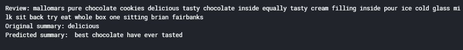
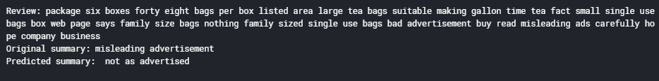
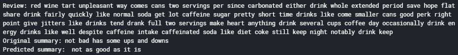
This is really cool stuff. Even though the actual summary and the summary generated by our model do not match in terms of words, both of them are conveying the same meaning. Our model is able to generate a legible summary based on the context present in the text.

This is how we can perform text summarization using deep learning concepts in Python.

How can we Improve the Model’s Performance Even Further?

Your learning doesn’t stop here! There’s a lot more you can do to play around and experiment with the model:

• I recommend you to increase the training dataset size and build the model. The generalization capability of a deep learning model enhances with an increase in the training dataset size
• Try implementing Bi-Directional LSTM which is capable of capturing the context from both the directions and results in a better context vector
• Use the beam search strategy for decoding the test sequence instead of using the greedy approach (argmax)
• Evaluate the performance of your model based on the BLEU score
• Implement pointer-generator networks and coverage mechanisms

How does the Attention Mechanism Work?

Now, let’s talk about the inner workings of the attention mechanism. As I mentioned at the start of the article, this is a math-heavy section so consider this as optional learning. I still highly recommend reading through this to truly grasp how attention mechanism works.

• The encoder outputs the hidden state (h j) for every time step j in the source sequence
• Similarly, the decoder outputs the hidden state (s i) for every time step i in the target sequence
• We compute a score known as an alignment score (eij) based on which the source word is aligned with the target word using a score function. The alignment score is computed from the source hidden state hj and target hidden state si using the score function. This is given by:

eij= score (si, hj )

where e ij denotes the alignment score for the target timestep i and source time step j.

There are different types of attention mechanisms depending on the type of score function used. I’ve mentioned a few popular attention mechanisms below:

• We normalize the alignment scores using softmax function to retrieve the attention weights (a ij):

• We compute the linear sum of products of the attention weights aij and hidden states of the encoder hj to produce the attended context vector (C i):

• The attended context vector and the target hidden state of the decoder at timestep i are concatenated to produce an attended hidden vector Si

Si= concatenate([si; Ci])

• The attended hidden vector Si is then fed into the dense layer to produce y i

yi= dense(Si)

Let’s understand the above attention mechanism steps with the help of an example. Consider the source sequence to be [x1, x2, x3, x4] and target sequence to be [y1, y2].

• The encoder reads the entire source sequence and outputs the hidden state for every timestep, say h1, h2, h3, h4

• The decoder reads the entire target sequence offset by one timestep and outputs the hidden state for every timestep, say s1, s2, s3

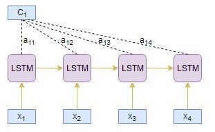
Target timestep i=1

• Alignment scores e1j are computed from the source hidden state hi and target hidden state s1 using the score function:

e11= score(s1, h1) e12= score(s1, h2) e13= score(s1, h3) e14= score(s1, h4)

• Normalizing the alignment scores e1j using softmax produces attention weights a1j:

a11= exp(e11)/((exp(e11)+exp(e12)+exp(e13)+exp(e14)) a12= exp(e12)/(exp(e11)+exp(e12)+exp(e13)+exp(e14)) a13= exp(e13)/(exp(e11)+exp(e12)+exp(e13)+exp(e14)) a14= exp(e14)/(exp(e11)+exp(e12)+exp(e13)+exp(e14))

• Attended context vector C 1 is derived by the linear sum of products of encoder hidden states h j and alignment scores a 1j:

C1= h1 * a11 + h2 * a12 + h3 * a13 + h4 * a14

• Attended context vector C1 and target hidden state s1 are concatenated to produce an attended hidden vector S1

S1= concatenate([s1; C1])

• Attentional hidden vector S1 is then fed into the dense layer to produce y 1

y1= dense(S1)

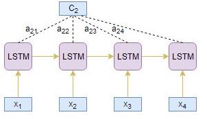
Target timestep i=2

• Alignment scores e2j are computed from the source hidden state hi and target hidden state s2 using the score function given by

e21= score(s2, h1) e22= score(s2, h2) e23= score(s2, h3) e24= score(s2, h4)

• Normalizing the alignment scores e 2j using softmax produces attention weights a 2j:

a21= exp(e21)/(exp(e21)+exp(e22)+exp(e23)+exp(e24)) a22= exp(e22)/(exp(e21)+exp(e22)+exp(e23)+exp(e24)) a23= exp(e23)/(exp(e21)+exp(e22)+exp(e23)+exp(e24)) a24= exp(e24)/(exp(e21)+exp(e22)+exp(e23)+exp(e24))

• Attended context vector C2 is derived by the linear sum of products of encoder hidden states hi and alignment scores a2j:

C2= h1 * a21 + h2 * a22 + h3 * a23 + h4 * a24

• Attended context vector C2 and target hidden state s2 are concatenated to produce an attended hidden vector S2

S2= concatenate([s2; C2])

• Attended hidden vector S2 is then fed into the dense layer to produce y2

y2= dense(S2)

We can perform similar steps for target timestep i=3 to produce y 3.

I know this was a heavy dosage of math and theory but understanding this will now help you to grasp the underlying idea behind attention mechanism. This has spawned so many recent developments in NLP and now you are ready to make your own mark!

Code

Find the entire notebook here.

Conclusion

Take a deep breath – we’ve covered a lot of ground in this article. And congratulations on building your first text summarization model using deep learning! We have seen how to build our own text summarizer using Seq2Seq modeling in Python.

If you have any feedback on this article or any doubts/queries, kindly share them in the comments section below and I will get back to you. And make sure you experiment with the model we built here and share your results with the community!

You can also take the below courses to learn or brush up your NLP skills:

• Natural Language Processing (NLP) using Python
• Introduction to Natural Language Processing (NLP)

Frequently Asked Questions

Q1. What is text summarization in NLP?

A. Text summarization in NLP (Natural Language Processing) involves using computational algorithms to automatically condense a large text document into a shorter summary that captures its essential information.

Q2. What are the 4 types of summarization?

A. The four types of summarization are: extraction, abstraction, indicative, and query-based. Extraction summarizes the most important information directly from the text. Abstraction summarizes information in a new way, while indicative focuses on the main message. Query-based uses specific questions to generate a summary.

Q3. Are there pre-trained models for text summarization?

Yes, pre-trained models like BERT, GPT, and T5 have been adapted for text summarization tasks, achieving state-of-the-art results due to their ability to capture contextual information.

Aravind Pai is passionate about building data-driven products for the sports domain. He strongly believes that Sports Analytics is a Game Changer.