Bayesian Optimization in Machine Learning (original) (raw)

Last Updated : 23 Jul, 2025

Bayesian Optimization is a powerful optimization technique that leverages the principles of Bayesian inference to find the minimum (or maximum) of an objective function efficiently. Unlike traditional optimization methods that require extensive evaluations, Bayesian Optimization is particularly effective when dealing with expensive, noisy, or black-box functions.

**This article delves into the core concepts, working mechanisms, advantages, and applications of Bayesian Optimization, providing a comprehensive understanding of why it has become a go-to tool for optimizing complex functions.

Table of Content

• What is Bayesian Optimization?
• How Does Bayesian Optimization Work?
• Key Concepts in Bayesian Optimization
• Advantages of Bayesian Optimization
• Applications of Bayesian Optimization
• Limitations of Bayesian Optimization
• Implementing Bayesian Optimization in Python
• Conclusion

What is Bayesian Optimization?

Bayesian Optimization is a strategy for optimizing expensive-to-evaluate functions. It operates by building a probabilistic model of the objective function and using this model to select the most promising points to evaluate next. This approach is particularly useful in scenarios where the objective function is unknown, noisy, or costly to evaluate, as it aims to minimize the number of evaluations required to find the optimal solution.

**The optimization process involves two main components:

1. **Surrogate Model: A probabilistic model (often a Gaussian Process) that approximates the objective function.
2. **Acquisition Function: A utility function that guides the selection of the next point to evaluate based on the surrogate model.

How Does Bayesian Optimization Work?

Bayesian optimization effectively combines statistical modeling and decision-making strategies to optimize complex, costly functions. Here’s a more detailed explanation of the process, including key formulas:

1. **Initialization

The process begins by sampling the objective function f at a few initial points. These points can be selected randomly or through systematic methods such as Latin Hypercube Sampling, which helps ensure diverse and comprehensive coverage of the input space.

2. **Building the Surrogate Model

A Gaussian Process (GP) is typically used as the surrogate model. The GP is favored for its ability to provide both a mean prediction and a measure of uncertainty (variance) at any point in the input space. The GP is defined by a mean function m(x) and a covariance function k(x, x'), and it models the function as:

f(x) \sim \mathcal{GP}(m(x), k(x, x'))

Where:

• m(x) is often assumed to be zero if no prior knowledge is available.
• k(x, x') is the kernel function that defines the covariance between any two points in the input space, such as the squared exponential kernel:

k(x, x') = \exp\left(-\frac{1}{2l^2} \| x - x' \|^2\right)

3. **Acquisition Function Maximization

The next sampling point is chosen by maximizing an acquisition function that trades off between exploration and exploitation. Common acquisition functions include:

• **Expected Improvement (EI):

EI(x) = \mathbb{E}\left[\max(f(x) - f(x^+), 0)\right]

Where f(x^+) is the current best observed value of f. EI measures the expected increase in the objective function relative to the best current observation.

• **Upper Confidence Bound (UCB):

UCB(x) = \mu(x) + \kappa \sigma(x)

Where \mu(x) and \sigma(x) are the mean and standard deviation of the GP’s predictions at point x, and \kappa is a parameter that balances exploration and exploitation.

4. **Evaluating the Objective Function

The point x selected by maximizing the acquisition function is then evaluated to obtain f(x). This new data point is added to the dataset, which is used to update the GP model.

5. **Iteration

The steps of updating the acquisition function, selecting new points, and updating the surrogate model are repeated. With each iteration, the surrogate model becomes increasingly accurate, and the search progressively hones in on the optimum.

6. **Termination

The optimization process continues until a predefined stopping criterion is met, such as reaching a maximum number of function evaluations or achieving a convergence threshold where the improvements become minimal.

This structured approach allows Bayesian optimization to efficiently navigate complex landscapes, minimizing the number of evaluations needed to locate the optimum by intelligently balancing exploration of unknown regions and exploitation of promising areas.

Key Concepts in Bayesian Optimization

1. **Gaussian Process (GP): A Gaussian Process is a non-parametric model that defines a distribution over functions. In Bayesian Optimization, GPs are often used as the surrogate model because they provide not only an estimate of the objective function but also a measure of uncertainty.
2. **Acquisition Functions:
   • **Expected Improvement (EI): A popular acquisition function that selects points where the expected improvement over the current best solution is maximized.
   • **Probability of Improvement (PI): Chooses points with the highest probability of improving the current best solution.
   • **Upper Confidence Bound (UCB): Balances exploration and exploitation by selecting points based on a confidence interval around the GP prediction.
3. **Exploration vs. Exploitation: Exploration involves searching in areas of the search space with high uncertainty, while exploitation focuses on areas where the surrogate model predicts good outcomes. The acquisition function manages this trade-off to efficiently find the optimum.

Advantages of Bayesian Optimization

• **Efficiency: Bayesian Optimization is highly efficient in finding the optimum with a minimal number of evaluations, making it ideal for expensive or time-consuming objective functions.
• **Flexibility: It can be applied to a wide range of optimization problems, including noisy, discontinuous, and non-convex functions, and is particularly well-suited for black-box optimization.
• **Uncertainty Quantification: The probabilistic nature of the surrogate model allows for uncertainty quantification, providing insights into the reliability of predictions and guiding the exploration of the search space.

Applications of Bayesian Optimization

• **Hyperparameter Tuning****:** In machine learning, Bayesian Optimization is widely used for hyperparameter tuning, where the objective function is often expensive to evaluate (e.g., training a deep learning model).
• **Robotics: In robotics, it is used to optimize control policies or parameters of a robot, where each evaluation might involve running a physical experiment.
• **Chemical Engineering: Bayesian Optimization helps in optimizing the design and control of chemical processes, where experimental evaluations are costly and time-consuming.
• **A/B Testing: In marketing and product design, Bayesian Optimization can be used to optimize A/B tests, where evaluating different versions of a product or strategy is expensive in terms of time and resources.
• **Simulations and Experiments: In scientific research, Bayesian Optimization is used to optimize simulations or physical experiments, where each run can be computationally expensive or time-consuming.

Limitations of Bayesian Optimization

• **Scalability: While effective for low to moderate-dimensional problems, Bayesian Optimization can struggle with high-dimensional spaces due to the complexity of the surrogate model.
• **Computational Overhead: The process of fitting the surrogate model and maximizing the acquisition function can be computationally intensive, especially as the number of evaluations increases.
• **Choice of Surrogate Model and Acquisition Function: The performance of Bayesian Optimization heavily depends on the choice of surrogate model and acquisition function, requiring careful consideration and tuning.

Implementing Bayesian Optimization in Python

In this section, we are going to implement Bayesian Optimization using the 'scikit-optimize' library in python.

You can install scikit-optimize using pip if you haven't already:

pip install scikit-optimize

• **Objective Function: This is the function you're trying to minimize, which takes a vector x as input and returns a scalar value. In this case, the function (x1 - 2)^2 + (x2 - 3)^2 is used as an example, with the minimum at (2, 3).
• **Search Space: The space defines the bounds for the parameters being optimized. Here, both x1 and x2 are real-valued and range between 0.0 and 5.0.
• **gp_minimize: This function from scikit-optimize performs Bayesian Optimization. The key arguments include the objective function, the search space, the number of function evaluations (n_calls), and a random state for reproducibility.
• **Result: The result of gp_minimize contains the best parameters found and the corresponding minimum value.
• **Plot Convergence: The convergence plot shows how the minimum value found by the optimization improves over time. Python `

import numpy as np from skopt import gp_minimize from skopt.space import Real, Integer from skopt.plots import plot_convergence

Define the objective function to minimize

def objective_function(x): return (x[0] - 2) ** 2 + (x[1] - 3) ** 2

Define the search space

space = [Real(0.0, 5.0, name='x1'), # Continuous space for x1 Real(0.0, 5.0, name='x2')] # Continuous space for x2

Perform Bayesian Optimization

result = gp_minimize(objective_function, # The function to minimize space, # The search space n_calls=20, # The number of evaluations random_state=42) # Random state for reproducibility

Print the best parameters and the corresponding minimum value

print("Best parameters: x1 = {:.4f}, x2 = {:.4f}".format(result.x[0], result.x[1])) print("Minimum value: {:.4f}".format(result.fun))

Plot convergence

plot_convergence(result)

`

**Output:

Best parameters: x1 = 2.0003, x2 = 3.0003
Minimum value: 0.0000

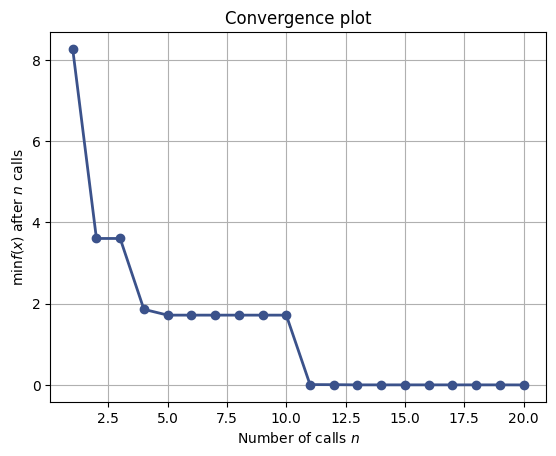
_The plot and the output together indicate that the Bayesian Optimization process was successful in finding the minimum of the objective function, and it converged efficiently after about 12 evaluations. The final solution is very close to the true minimum of the function, as indicated by the near-zero minimum value.

Conclusion

Bayesian Optimization stands out as a powerful and efficient approach to optimizing complex functions, particularly when evaluations are expensive, noisy, or time-consuming. Its ability to balance exploration and exploitation through a probabilistic surrogate model makes it a versatile tool across various domains, from machine learning to scientific research. By understanding and implementing Bayesian Optimization, practitioners can achieve optimal solutions with minimal evaluations, saving both time and resources in the process.