Classical Planning in AI (original) (raw)
Last Updated : 7 Nov, 2025
Classical Planning is a fundamental concept in Artificial Intelligence (AI) that focuses on finding an optimal sequence of actions to reach a desired goal from an initial state. It assumes a deterministic, fully observable and static environment where the agent knows exactly how each action affects the world. It contains:
- **State: Represents the configuration of the world at a specific time i.e all facts that are currently true.
- **Action: Defines transitions between states. Each action has Preconditions (what must be true before it executes.) and Effect (show the action changes the world.).
- **Goal: The desired end-state that satisfies the planner’s objective.
- **Plan: A sequence of actions that transitions the system from the initial state to the goal while satisfying all constraints.
It plays an important role in robotics, automated problem-solving, logistics and game AI which helps systems act intelligently and efficiently by reasoning about the outcomes of actions.
Domain-Independent Planning
One of the strengths of Classical Planning is its domain independence. This means planning techniques can be used in many different fields without adjusting the core methods. This makes classical planning highly flexible and widely applicable.
Domain-independent planning focuses on the key aspects of any planning problem like:
- **State representations: How to describe the current situation.
- **Action models: How actions can change the state.
- **Search strategy: How to systematically find the sequence of actions that lead to the goal.
By using general principles rather than relying on detailed knowledge of a specific domain, these methods can be applied across many different fields including robotics, logistics, manufacturing and more.
Planning Domain Modelling Languages
The domain independence in classical planning can be further understood through the use of domain-independent modelling languages such as PDDL (Planning Domain Definition Language) and STRIPS (Stanford Research Institute Problem Solver). These languages allow planners to represent problems in a way that is not tied to any specific domain, making them applicable to a variety of planning tasks.
- **PDDL (Planning Domain Definition Language): It is used for describing the objects, actions and goals in a planning problem. It provides a flexible framework to define both simple and complex planning scenarios.
- **STRIPS (Stanford Research Institute Problem Solver): It is one of the earliest planning languages that introduced a way to represent the state of the world, actions and the effects of those actions. It laid the foundation for many modern planning systems.
Classical Planning Techniques
Classical planning assumes a static and fully observable environment where the goal is to find a sequence of actions to move from the current state to the goal state while satisfying any constraints. There are two main categories of planning techniques:
1. State-Space Search
State-space search explores the space of all possible states by applying actions step-by-step until the goal is reached.
**Key Algorithms
- **Breadth-First Search (BFS)****:** Explores all nodes at the current depth before moving deeper. It guarantees the shortest path but can be memory-intensive.
- **Depth-First Search (DFS)****:** Explores deeply first and it uses less memory but may miss the optimal solution.
- **A* and **Greedy Search****:** Use heuristics to guide the search hence improving efficiency.
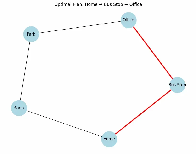
Let's see an example of breadth-first search in Python:
- **queue = deque([[start]]): Stores possible paths beginning from the start node.
- **visited: Keeps track of explored states to avoid loops.
- Each iteration checks neighbors and extends the path until the goal is found.
- The final red path in the visualization represents the shortest route from start to goal. Python `
from collections import deque import networkx as nx import matplotlib.pyplot as plt
class BFSPlanner: def init(self, graph): self.graph = graph
def plan(self, start, goal):
    """Finds the shortest plan from start to goal."""
    queue = deque([[start]])
    visited = set()

    while queue:
        path = queue.popleft()
        state = path[-1]

        if state == goal:
            return path

        if state not in visited:
            visited.add(state)
            for neighbor in self.graph.get(state, []):
                new_path = list(path)
                new_path.append(neighbor)
                queue.append(new_path)
    return None

def visualize_plan(self, path):
    """Draws the graph with the discovered path highlighted."""
    G = nx.Graph(self.graph)
    pos = nx.spring_layout(G, seed=42)
    plt.figure(figsize=(8, 6))
    nx.draw(G, pos, with_labels=True, node_color="lightblue",
            node_size=2200, font_size=12)
    if path:
        edges = [(path[i], path[i + 1]) for i in range(len(path) - 1)]
        nx.draw_networkx_edges(
            G, pos, edgelist=edges, edge_color="red", width=3)
        plt.title(f"Optimal Plan: {' → '.join(path)}", fontsize=13)
    plt.show()
world = { 'Home': ['Bus Stop', 'Shop'], 'Bus Stop': ['Home', 'Office'], 'Shop': ['Home', 'Park'], 'Park': ['Shop', 'Office'], 'Office': ['Bus Stop', 'Park'] }
planner = BFSPlanner(world) path = planner.plan('Home', 'Office') print("Generated Plan:", path) planner.visualize_plan(path)
`
**Output:
Output
State-space search is ideal for pathfinding and problems where the goal is to find the most efficient route.
2. Plan-Space Search
Plan-space search starts with a partial plan and incrementally refines it until it’s complete and consistent. This approach is useful for problems with complex dependencies between actions.
**Techniques Include
- **Partial-Order Planning (POP): Keeps flexibility in action order, specifying only necessary dependencies.
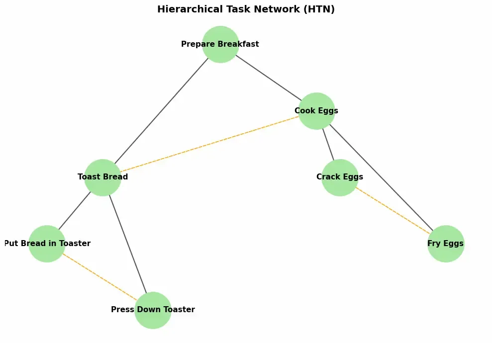
- **Hierarchical Task Network (HTN) Planning: HTN breaks complex tasks into simpler subtasks using a hierarchical decomposition approach.
- **UCPOP / VHPOP: Use refinement and constraint resolution to complete plans.
Let's see an example of Hierarchical Task Network in Python:
- decompose() recursively expands complex tasks into primitive subtasks.
- generate_plan() reverses the plan to ensure logical execution order.
- The visual shows hierarchical decomposition (solid arrows) and task sequence flow (dashed arrows). Python `
import networkx as nx import matplotlib.pyplot as plt
class HTNPlanner: def init(self, tasks): self.tasks = tasks self.plan = []
def decompose(self, task):
    """Recursively breaks down tasks into primitive actions."""
    if task not in self.tasks:
        self.plan.append(task)
        return
    for subtask in self.tasks[task]:
        self.decompose(subtask)
    self.plan.append(task)

def generate_plan(self, root):
    self.plan.clear()
    self.decompose(root)
    return self.plan[::-1]

def visualize(self, root):
    """Visualize HTN as a hybrid hierarchy + flow chart."""
    G = nx.DiGraph()

    for parent, children in self.tasks.items():
        for i, child in enumerate(children):
            G.add_edge(parent, child)
            if i < len(children) - 1:
                G.add_edge(children[i], children[i + 1], style="dashed")

    pos = nx.nx_agraph.graphviz_layout(G, prog="dot")
    plt.figure(figsize=(10, 7))

    solid_edges = [(u, v) for u, v, d in G.edges(
        data=True) if d.get("style") != "dashed"]
    dashed_edges = [(u, v) for u, v, d in G.edges(
        data=True) if d.get("style") == "dashed"]

    nx.draw_networkx_edges(G, pos, edgelist=solid_edges,
                           arrows=True, arrowstyle="-|>", arrowsize=15, width=1.5)
    nx.draw_networkx_edges(G, pos, edgelist=dashed_edges,
                           arrows=True, style="dashed", edge_color="orange")

    nx.draw_networkx_nodes(G, pos, node_color="#A6E7A1", node_size=2800)
    nx.draw_networkx_labels(G, pos, font_size=11, font_weight="bold")
    plt.title("Hierarchical Task Network (HTN)",
              fontsize=14, fontweight="bold")
    plt.axis("off")
    plt.tight_layout()
    plt.show()
htn_tasks = { "Prepare Breakfast": ["Cook Eggs", "Toast Bread"], "Cook Eggs": ["Crack Eggs", "Fry Eggs"], "Toast Bread": ["Put Bread in Toaster", "Press Down Toaster"] }
planner = HTNPlanner(htn_tasks) plan = planner.generate_plan("Prepare Breakfast") print("HTN Plan:", " → ".join(plan)) planner.visualize("Prepare Breakfast")
`
**Output:
Output
Plan-space search is best for tasks that involve complex action sequences or dependencies.
Reducing Classical Planning to Other Problems
Classical planning can be made more efficient by transforming it into well-established problems in computer science such as satisfiability (SAT) and constraint satisfaction problems (CSP). By using specialized solvers developed for these problems, planning tasks can be solved more effectively.
- **SAT-based Planning: Converts planning problems into propositional logic formulas solved by SAT solvers.
- **CSP-based Planning: Models the problem as a constraint satisfaction task with preconditions, effects and goal constraints.
Applications
Classical planning is useful in a variety of domains including:
- **Robotics: Path and action sequence planning for autonomous robots.
- **Automated Scheduling: Resource allocation and process scheduling.
- **Game AI: NPCs use planners to decide logical action sequences.
- **Space Missions: Autonomous planning for rover operations and satellite control.
Advantages
- **Optimality: Finds the shortest or most efficient sequence.
- **Simplicity: Easy to understand and implement.
- **Structured Problem Definition: Clear initial and goal states.
- **Domain Independence: Works across varied fields with the same principles.
Limitations
- **State Space Explosion: Exponential growth in possible states.
- **Static Assumptions: Assumes a deterministic, fully observable environment.
- **No Temporal Dynamics: Doesn’t model action durations or concurrency.
- **Limited Flexibility: Struggles with uncertainty or incomplete knowledge.