Diffusion Models in Machine Learning (original) (raw)

Last Updated : 1 Apr, 2026

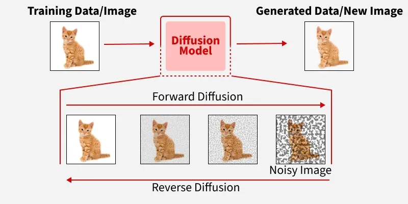
Diffusion Models in Machine Learning are generative models that create new data by learning to reverse a process of gradually adding noise to training samples. They use neural networks and probabilistic principles to transform random noise into realistic, high-quality outputs. These models are widely applied in tasks like image generation, inpainting and super-resolution, capturing complex data patterns.

• Training involves modeling the gradual transformation of data through multiple intermediate steps.
• Performance improves with larger datasets and longer denoising sequences.
• Adaptable for extensions like conditional generation and cross-modal tasks.

Diffusion Models

How it Works

Diffusion Models generate data by progressively transforming noise into structured outputs. This process can be divided into four components.

• The noise schedule is crucial for training it determines how quickly data is corrupted and affects sample quality.
• Diffusion models typically require many steps for the forward and reverse processes to ensure smooth data reconstruction.
• Variants like conditional diffusion models allow guidance with extra information, such as text prompts for image generation.

1. Forward Process

The forward process gradually adds Gaussian noise to a data sample x0 over several steps until it becomes nearly pure noise. This defines a sequence of noisy versions x1, x2, ..., xT that the model will learn to reverse.

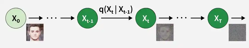
Forward Diffusion

Forward diffusion process is represented using a distribution q, which describes how noise is added at each step.

q(x_t \mid x_{t-1}) = \mathcal{N}\left(x_t;\sqrt{1-\beta_t}\,x_{t-1},\,\beta_t I\right)

Where

• x_{t-1}: Data at the previous time step
• x_{t}: Data at the current time step after adding noise
• \beta_{t}: Variance schedule controlling how much noise is added at step t
• I: Identity matrix
• \mathcal{N}: Gaussian (normal) distribution

As t increases, xt transitions from the original data x0 to pure noise. The forward process defines the probability distribution that the model will learn to reverse.

2. Reverse Process

The reverse process reconstructs the original data from noisy inputs by predicting the clean sample at each step. This is modeled using a neural network that estimates the distribution of the previous step conditioned on the current noisy data.

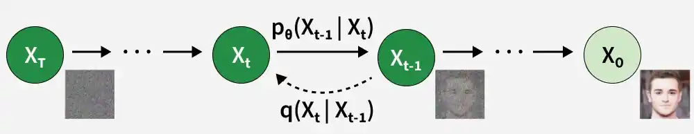
Reverse Diffusaion

p(x_{t-1} \mid x_t) = \mathcal{N}\big(x_{t-1}; \mu_\theta(x_t, t), \sigma_t^2 \mathbf{I} \big)

Where

• \mu_{\theta}(x_{t},t) is the mean predicted by the neural network
• \sigma_{t}^{2} is the variance at step t

The reverse process is applied iteratively, step by step gradually converting noise into high-quality structured data.

3. Training the Model

Training a diffusion model involves optimizing the neural network to predict the noise added during the forward process. The network learns to minimize the difference between predicted noise and actual noise, effectively learning how to reverse the diffusion.

L(\theta) = \mathbb{E}_{x_0, \epsilon, t} \big[ \| \epsilon - \epsilon_\theta(x_t, t) \|^2 \big]

Where

• \epsilon is the actual noise
• \epsilon_{\theta}(x_{t},t) is the predicted noise by the network

This optimization allows the model to reconstruct realistic data from random noise after training.

4. Score Matching

Some diffusion models use score matching, which estimates the gradient of the log probability density (the score function). This helps improve the accuracy of the reverse process by better approximating the underlying data distribution.

• Score matching provides a probabilistic foundation for reversing noise.
• Enables more stable and high-quality sample generation.
• Often used in continuous-time diffusion models and variants like DDPMs (Denoising Diffusion Probabilistic Models).

L_{\text{score}}(\theta) = \mathbb{E}_{x_0, t} \Big[ \big\| \nabla_{x_t} \log p(x_t \mid x_0) - \nabla_{x_t} \log p_\theta(x_t) \big\|^2 \Big]

Step By Step Implementation

Step 1: Import Required Libraries

• **torch: Core PyTorch library used for tensor operations and deep learning computations.
• **torch.nn: Provides neural network layers and model-building utilities.
• **torch.nn.functional: Contains activation functions and loss functions.
• **torchvision: Used for loading datasets like CIFAR-10.
• **torchvision.transforms: Applies preprocessing and normalization to images.
• **DataLoader: Handles batching and shuffling of dataset during training. Python `

import torch import torch.nn as nn import torch.nn.functional as F import torchvision import torchvision.transforms as transforms from torch.utils.data import DataLoader import matplotlib.pyplot as plt import numpy as np

device = torch.device("cuda" if torch.cuda.is_available() else "cpu")

`

Step 2: Define Hyperparameters and Noise Schedule

Batch size, epochs, learning rate and total diffusion steps are defined and beta, alpha and cumulative alpha (\alpha) values are computed to control the gradual addition of noise during diffusion.

Python `

batch_size = 128 epochs = 150 lr = 1e-4 T = 1000

beta = torch.linspace(1e-4, 0.02, T).to(device) alpha = 1. - beta alpha_hat = torch.cumprod(alpha, dim=0)

`

Step 3: Implement Sinusoidal Time Embedding

Sinusoidal position embeddings are used to encode timestep information so the model can understand the diffusion stage.

• The class inherits from nn.Module and takes embedding dimension dim as input.
• Exponential scaling is applied using torch.exp and logarithmic spacing to generate frequency components.
• Sine and cosine functions are combined to produce a continuous, smooth timestep representation. Python `

class SinusoidalPositionEmbeddings(nn.Module): def init(self, dim): super().init() self.dim = dim

def forward(self, time):
    device = time.device
    half_dim = self.dim // 2
    embeddings = torch.exp(
        torch.arange(half_dim, device=device) * 
        -(np.log(10000) / (half_dim - 1))
    )
    embeddings = time[:, None] * embeddings[None, :]
    embeddings = torch.cat((embeddings.sin(), embeddings.cos()), dim=-1)
    return embeddings

`

Step 4: Build the Denoising Neural Network

A convolutional neural network is defined to predict the noise added at each diffusion timestep.

• time_mlp processes sinusoidal timestep embeddings through a linear layer and ReLU activation to generate time-aware features.
• Three convolutional layers extract image features, where timestep information is added to the first feature map for conditioning.
• The model predicts noise with the final convolution layer, and the Adam optimizer is initialized for training. Python `

class Denoiser(nn.Module): def init(self): super().init() self.time_mlp = nn.Sequential( SinusoidalPositionEmbeddings(32), nn.Linear(32, 64), nn.ReLU() )

    self.conv1 = nn.Conv2d(3, 64, 3, padding=1)
    self.conv2 = nn.Conv2d(64, 64, 3, padding=1)
    self.conv3 = nn.Conv2d(64, 3, 3, padding=1)

def forward(self, x, t):
    t = self.time_mlp(t)
    t = t[:, :, None, None]
    x = self.conv1(x)
    x = x + t
    x = F.relu(self.conv2(x))
    return self.conv3(x)

model = Denoiser().to(device) optimizer = torch.optim.Adam(model.parameters(), lr=lr)

`

Step 5: Load and Preprocess CIFAR-10 Dataset

CIFAR-10 images are converted to tensors and normalized to the range [-1, 1] for stable training. The DataLoader creates shuffled batches to efficiently feed data into the model during training.

Python `

transform = transforms.Compose([ transforms.ToTensor(), transforms.Normalize((0.5,), (0.5,)) ])

dataset = torchvision.datasets.CIFAR10( root='./data', train=True, download=True, transform=transform )

dataloader = DataLoader(dataset, batch_size=batch_size, shuffle=True)

`

Step 6: Implement Forward Diffusion Process

Gaussian noise is added to clean images using cumulative alpha (\alpha) values according to the diffusion equation. The function returns the noisy image at timestep t along with the generated noise used for training.

Python `

def forward_diffusion(x0, t): noise = torch.randn_like(x0) sqrt_alpha_hat = torch.sqrt(alpha_hat[t])[:, None, None, None] sqrt_one_minus_alpha_hat = torch.sqrt(1 - alpha_hat[t])[:, None, None, None] return sqrt_alpha_hat * x0 + sqrt_one_minus_alpha_hat * noise, noise

`

Step 7: Train the Diffusion Model

The model is trained to predict the noise added at random diffusion timesteps using mean squared error loss.

• For each batch, a random timestep t is sampled and noise is added using the forward diffusion function.
• The model predicts the added noise from the noisy image and MSE loss is computed between predicted and true noise.
• Gradients are calculated using backpropagation and the optimizer updates model parameters after each iteration. Python `

for epoch in range(epochs): for images, _ in dataloader: images = images.to(device) t = torch.randint(0, T, (images.size(0),), device=device)

    xt, noise = forward_diffusion(images, t)

    predicted_noise = model(xt, t.float())
    loss = F.mse_loss(predicted_noise, noise)

    optimizer.zero_grad()
    loss.backward()
    optimizer.step()

print(f"Epoch {epoch+1}, Loss: {loss.item()}")

print("Training completed!")

`

**Output:

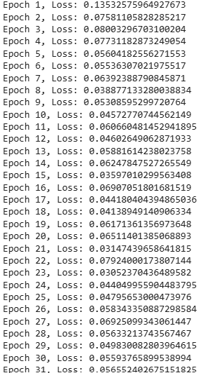
Model Traning

Step 8: Reverse Diffusion and Image Generation

The reverse diffusion process generates new images by gradually removing noise from random input samples using the trained model.

• The function starts with random Gaussian noise and iteratively applies the reverse diffusion formula from timestep T down to 0.
• At each step, the model predicts the noise, which is used along with alpha and beta values to update the image.
• After sampling, generated images are rescaled to the range [0, 1]. Python `

def sample(model, n): model.eval() x = torch.randn((n, 3, 32, 32)).to(device)

for t in reversed(range(T)):
    t_tensor = torch.full((n,), t, device=device)
    predicted_noise = model(x, t_tensor.float())

    alpha_t = alpha[t]
    alpha_hat_t = alpha_hat[t]
    beta_t = beta[t]

    if t > 0:
        noise = torch.randn_like(x)
    else:
        noise = torch.zeros_like(x)

    x = (1 / torch.sqrt(alpha_t)) * (
        x - (1 - alpha_t) / torch.sqrt(1 - alpha_hat_t) * predicted_noise
    ) + torch.sqrt(beta_t) * noise

return x

generated_images = sample(model, 8) generated_images = (generated_images + 1) / 2 generated_images = generated_images.clamp(0,1).detach().cpu()

plt.figure(figsize=(12,4)) for i in range(8): plt.subplot(1,8,i+1) plt.imshow(generated_images[i].permute(1,2,0)) plt.axis('off') plt.show()

`

**Output:

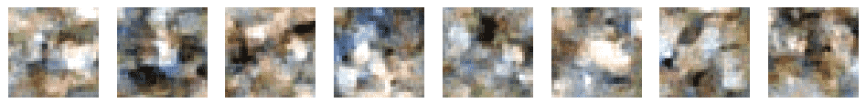
Generated Image

Step 9: Visualize the Forward Noising Process

A sample image is selected and progressively noised at different timesteps to show how the diffusion process gradually corrupts the original image from clean data to nearly pure noise.

Python `

sample_img, _ = dataset[0] sample_img = sample_img.unsqueeze(0).to(device)

plt.figure(figsize=(12,3)) for i, step in enumerate([0, 50, 100, 200, 299]): t = torch.tensor([step], device=device) xt, _ = forward_diffusion(sample_img, t) xt = (xt + 1) / 2 xt = xt.clamp(0,1).cpu() plt.subplot(1,5,i+1) plt.imshow(xt[0].permute(1,2,0)) plt.title(f"t={step}") plt.axis('off') plt.show()

`

**Output:

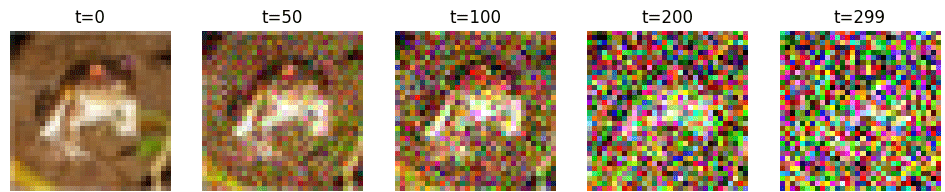
Output

Download full code from here.

Applications

Diffusion models have found numerous applications in machine learning, including:

1. **Image Processing: Enhancing image quality through techniques like denoising and super-resolution where diffusion models help in smoothing out noise and improving resolution.
2. **Natural Language Processing (NLP): Understanding and generating text by modeling the diffusion of semantic information. Diffusion models can be used for tasks such as text generation, sentiment analysis and topic modeling.
3. **Predictive Modeling and Time Series Analysis: Forecasting future trends and behaviors in time series data, such as stock prices, weather patterns and epidemiological trends. Diffusion models can capture the temporal dependencies and make accurate predictions.
4. **Biomedical Applications: Modeling the spread of diseases, analyzing brain connectivity and studying genetic data. Diffusion models contribute to advancements in medical diagnostics and treatment planning.
5. **Social Network Analysis: Studying the spread of information, influenc and behaviors in social networks. Diffusion models help identify influential nodes, predict viral content and understand community dynamics.

Advantages

• Produce high-quality and highly realistic samples that closely resemble real data, often outperforming traditional generative models such as GANs in visual fidelity.
• Provide a more stable and reliable training process compared to adversarial models, reducing issues like mode collapse.
• Support strong diversity in generated outputs while maintaining consistency with the learned data distribution.
• Apply to multiple data modalities, including images, audio, video and multimodal generation tasks.

Limitations

• Training and sampling processes are computationally expensive and time-consuming due to the large number of diffusion steps required.
• Generating high-resolution images or handling very large datasets demands significant GPU memory and processing power.
• Inference (image generation) is slower compared to some other generative models because it requires iterative denoising over many steps.
• Model performance is sensitive to the choice of noise schedule and hyperparameters, requiring careful tuning.