LeNet5 Architecture (original) (raw)
LeNet-5 Architecture
Last Updated : 18 May, 2026
LeNet-5 is a convolutional neural network (CNN) designed for image recognition, especially handwritten digit classification. It introduced a structured approach to feature learning in neural networks.
- Uses convolution and pooling layers for feature extraction.
- Applies hierarchical learning from simple to complex patterns.
- Simple and efficient architecture suitable for small datasets.
Architecture of LeNet-5
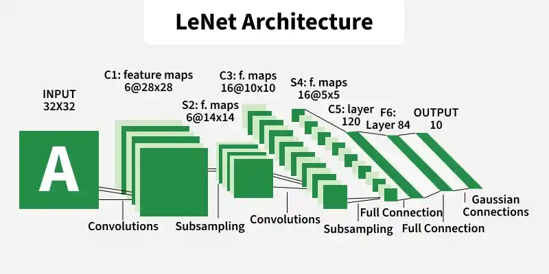
Architecture
1. Input Layer
- **Input size: 32×32 grayscale image.
- **Padding: Ensures important features are centered and captured effectively.
- **Normalization: Scales pixel values (0–1) for stable and faster training.
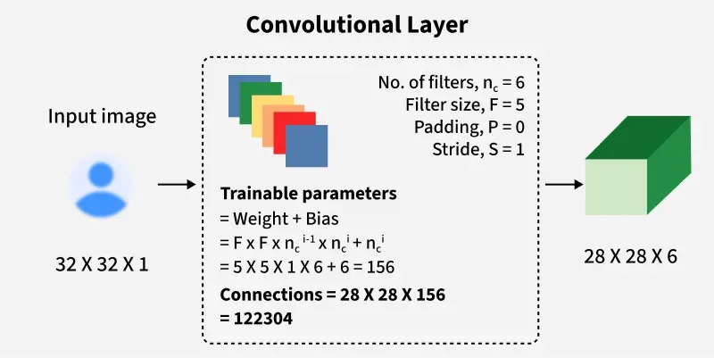
2. **Layer C1 (Convolutional Layer)
- **Feature Maps: 6 feature maps.
- **Connections: Each unit is connected to a 5x5 neighborhood in the input, producing 28x28 feature maps to prevent boundary effects.
- **Parameters: 156 trainable parameters and 117,600 connections.
First Layer
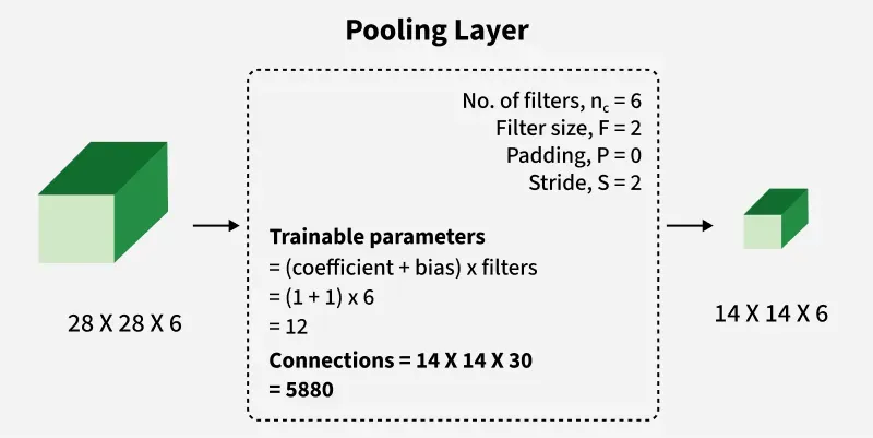
**3. Layer S2 (Subsampling Layer)
- **Feature Maps: 6 feature maps.
- **Size: 14x14 (each unit connected to a 2x2 neighborhood in C1).
- **Operation: Each unit adds four inputs, multiplies by a trainable coefficient, adds a bias, and applies a sigmoid function.
- **Parameters: 12 trainable parameters and 5,880 connections.
Second Layer
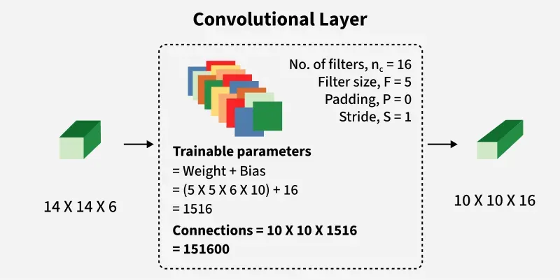
**Partial Connectivity: C3 is not fully connected to S2, which limits the number of connections and breaks symmetry, forcing feature maps to learn different, complementary features.
4. **Layer C3 (Convolutional Layer)
- **Feature Maps: 16 feature maps for learning patterns.
- **Kernel Size: 5×5 filters for feature extraction.
- **Connections: Partially connected to previous layer.
- **Parameters: 1,516 trainable parameters.
- **Partial Connectivity: Reduces parameters and encourages diverse feature learning.
Third Layer
5. **Layer S4 (Subsampling Layer)
- **Feature Maps: 16 feature maps.
- **Size: 7x7 feature map size
- **Parameters: 32 trainable parameters and 2,744 connections.
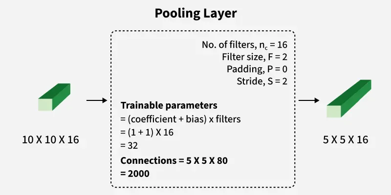
Fourth Layer
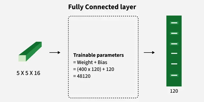
6. **Layer C5 (Convolutional Layer)
- **Feature Maps: 120 feature maps.
- **Size: 1×1 feature map size.
- **Connections: Fully connected to all previous feature maps.
- **Parameters: 48,000 trainable parameters.
Fifth Layer
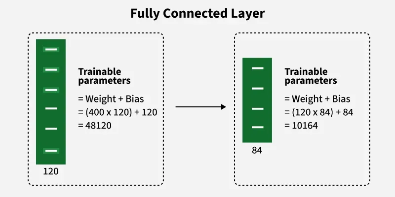
7. **Layer F6 (Fully Connected Layer)
- **Units: 84 units.
- **Connections: Each unit is fully connected to C5, resulting in 10,164 trainable parameters.
- **Activation: Uses a scaled hyperbolic tangent function f(a) = A\tan (Sa), where A = 1.7159 and S = 2/3
Sixth Layer
8. **Output Layer
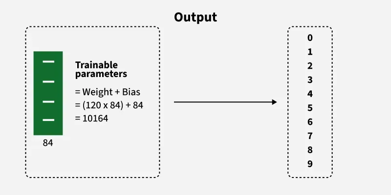
Output Layer
In the output layer of LeNet, each class is represented by a Radial Basis Function (RBF) unit, where the output depends on the Euclidean distance between the input and its parameter vector, with larger distances indicating poorer fit.
Here's how the output of each RBF unit y_iis computed:
y_i = \sum_{j} x_j . w_{ij}
In this equation:
- x_j represents the inputs to the RBF unit.
- w_{ij} represents the weights associated with each input.
- The summation is over all inputs to the RBF unit.
Implementation
1. Loading the Dataset
Load the MNIST dataset for training and testing the model.
Python `
import matplotlib.pyplot as plt import tensorflow as tf import numpy as np
mnist = tf.keras.datasets.mnist (x_train, y_train), (x_test, y_test) = mnist.load_data()
`
2. Pre-processing and Normalizing the Data
Reshape and normalize images, and convert labels into one-hot encoding.
Python `
rows, cols = 28, 28
Reshape the data into a 4D Array
x_train = x_train.reshape(x_train.shape[0], rows, cols, 1) x_test = x_test.reshape(x_test.shape[0], rows, cols, 1)
input_shape = (rows,cols,1)
Set type as float32 and normalize the values to [0,1]
x_train = x_train.astype('float32') x_test = x_test.astype('float32') x_train = x_train / 255.0 x_test = x_test / 255.0
Transform labels to one hot encoding
y_train = tf.keras.utils.to_categorical(y_train, 10)
`
3. Define LeNet-5 Model
Creates a Sequential model, adds LeNet-5 layers, and compiles it using categorical cross-entropy loss, SGD optimizer, and accuracy metric.
Each MNIST image is 28×28 pixels, so LeNet-5 is adapted to use 28×28 input instead of 32×32.
Python `
def build_lenet(input_shape):
Define Sequential Model
model = tf.keras.Sequential()
C1 Convolution Layer
model.add(tf.keras.layers.Conv2D(filters=6, strides=(1,1), kernel_size=(5,5), activation='tanh', input_shape=input_shape))
S2 SubSampling Layer
model.add(tf.keras.layers.AveragePooling2D(pool_size=(2,2), strides=(2,2)))
C3 Convolution Layer
model.add(tf.keras.layers.Conv2D(filters=6, strides=(1,1), kernel_size=(5,5), activation='tanh'))
S4 SubSampling Layer
model.add(tf.keras.layers.AveragePooling2D(pool_size=(2,2), strides=(2,2)))
C5 Fully Connected Layer
model.add(tf.keras.layers.Dense(units=120, activation='tanh'))
Flatten the output so that we can connect it with the fully connected layers by converting it into a 1D Array
model.add(tf.keras.layers.Flatten())
FC6 Fully Connected Layers
model.add(tf.keras.layers.Dense(units=84, activation='tanh'))
Output Layer
model.add(tf.keras.layers.Dense(units=10, activation='softmax'))
return model
`
4. Evaluate the Model and Visualize the process
- Uses
model.fit()with training data, epochs, and batch size. - Validation is performed using
validation_splitorvalidation_datato monitor performance after each epoch. - Evaluation is done using
model.evaluate()on the test dataset. - Training progress is visualized using accuracy and loss plots. Python `
lenet = build_lenet(input_shape)
Compile the model
lenet.compile(optimizer='adam', loss='categorical_crossentropy', metrics=['accuracy'])
We will be allowing 10 itterations to happen
epochs = 10 history = lenet.fit(x_train, y_train, epochs=epochs,batch_size=128, verbose=1)
Check Accuracy of the Model
Transform labels to one hot encoding
if len(y_test.shape) != 2 or y_test.shape[1] != 10: y_test = tf.keras.utils.to_categorical(y_test, 10)
loss ,acc= lenet.evaluate(x_test, y_test) print('Accuracy : ', acc)
x_train = x_train.reshape(x_train.shape[0], 28,28) print('Training Data', x_train.shape, y_train.shape) x_test = x_test.reshape(x_test.shape[0], 28,28) print('Test Data', x_test.shape, y_test.shape)
Plot the Image
image_index = 8888 plt.imshow(x_test[image_index].reshape(28,28), cmap='Greys')
Make Prediction
pred = lenet.predict(x_test[image_index].reshape(1, rows, cols, 1 )) print(pred.argmax())
`
**Output:
Epoch 1/10 469/469 ━━━━━━━━━━━━━━━━━━━━ 29s 55ms/step - accuracy: 0.8350 - loss: 0.5978
Epoch 2/10 469/469 ━━━━━━━━━━━━━━━━━━━━ 21s 44ms/step - accuracy: 0.9511 - loss: 0.1647
Epoch 3/10 469/469 ━━━━━━━━━━━━━━━━━━━━ 42s 46ms/step - accuracy: 0.9668 - loss: 0.1143
Epoch 4/10 469/469 ━━━━━━━━━━━━━━━━━━━━ 25s 54ms/step - accuracy: 0.9750 - loss: 0.0853
Epoch 5/10 469/469 ━━━━━━━━━━━━━━━━━━━━ 39s 50ms/step - accuracy: 0.9794 - loss: 0.0702
Epoch 6/10 469/469 ━━━━━━━━━━━━━━━━━━━━ 40s 48ms/step - accuracy: 0.9840 - loss: 0.0567
Epoch 7/10 469/469 ━━━━━━━━━━━━━━━━━━━━ 21s 46ms/step - accuracy: 0.9844 - loss: 0.0514
Epoch 8/10 469/469 ━━━━━━━━━━━━━━━━━━━━ 41s 46ms/step - accuracy: 0.9871 - loss: 0.0429
Epoch 9/10 469/469 ━━━━━━━━━━━━━━━━━━━━ 40s 43ms/step - accuracy: 0.9886 - loss: 0.0388
Epoch 10/10 469/469 ━━━━━━━━━━━━━━━━━━━━ 22s 46ms/step - accuracy: 0.9901 - loss: 0.0335
313/313 ━━━━━━━━━━━━━━━━━━━━ 2s 6ms/step - accuracy: 0.9796 - loss: 0.0544
Accuracy : 0.9832000136375427
Training Data (60000, 28, 28) (60000, 10)
Test Data (10000, 28, 28) (10000, 10)
1/1 ━━━━━━━━━━━━━━━━━━━━ 0s 108ms/step
6
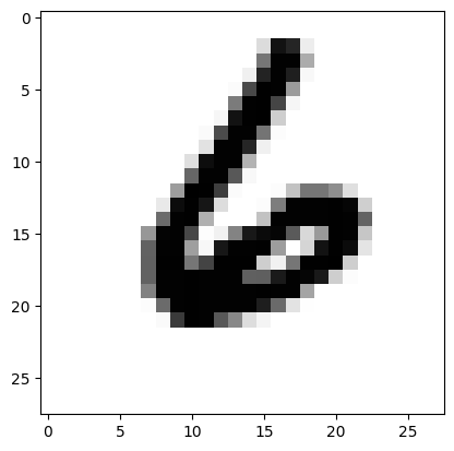
Output - LeNet5
Summary of LeNet-5 Architecture
| Layer | Feature Maps | Size | Kernel | Stride | Activation |
|---|---|---|---|---|---|
| Input | 1 | 32×32 | - | - | - |
| Conv1 | 6 | 28×28 | 5×5 | 1 | tanh |
| Avg Pool | 6 | 14×14 | 2×2 | 2 | tanh |
| Conv2 | 16 | 10×10 | 5×5 | 1 | tanh |
| Avg Pool | 16 | 5×5 | 2×2 | 2 | tanh |
| Conv3 | 120 | 1×1 | 5×5 | 1 | tanh |
| FC | 84 | - | - | - | tanh |
| Output | 10 | - | - | - | softmax |