What are the main steps in a typical Computer Vision Pipeline? (original) (raw)

Last Updated : 11 Aug, 2025

Computer vision is a field of artificial intelligence (AI) that enables machines to interpret and understand the visual world. By using digital images from cameras and videos and deep learning models, machines can accurately identify and classify objects and then react to what they “see.” A computer vision pipeline outlines the steps required to process and analyze visual data. Here, we delve into the main steps of a typical computer vision pipeline.

1. Image Acquisition

Collect raw data with digital cameras, webcams, CCTV systems, smartphones, drones, satellites, X-ray, MRI or microscopy devices. Use still images, video frames or multi-spectral formats. Consider lighting, object position, environmental factors, sensor calibration, frame rate and image resolution at this stage.

**Devices Used: Cameras, smartphones, drones, satellite imagery and medical imaging devices.
**Considerations: Lighting conditions, focus, frame rate and resolution. Python `

import cv2 img = cv2.imread('sample_image.jpg') if img is None: raise FileNotFoundError( "sample_image.jpg not found. Please upload an image with this name.")

Loads an image named "sample_image.jpg". If the image is not found, the program exits with an error message.

To download the used sample, click here.

2. Preprocessing

Noise Reduction: Applying filters (e.g., Gaussian filter) to remove noise from the image.
Normalization: Adjusting the intensity values to a common scale, often between 0 and 1.
Image Scaling: Resizing images to a fixed dimension required by the model.
Data Augmentation: Techniques like rotation, flipping, cropping and color adjustments to artificially expand the dataset. Python `

img_blur = cv2.GaussianBlur(img, (5, 5), 0) img_resized = cv2.resize(img_blur, (224, 224)) img_normalized = img_resized / 255.0 from torchvision import transforms transform = transforms.Compose([ transforms.ToPILImage(), transforms.RandomHorizontalFlip(), transforms.RandomRotation(10), transforms.ToTensor() ]) img_tensor = transform(img_normalized.astype('float32')) img_tensor = torch.unsqueeze(img_tensor, 0)

Applies Gaussian blur for noise reduction, resizes the image to 224×224 pixels for deep learning model compatibility, normalizes pixel values and augments data using flip and rotation. Converts image to tensor format for model input.

3. Image Segmentation

Apply simple thresholding (e.g., Otsu’s method), adaptive thresholding or edge detectors like Canny, Sobel, Prewitt or Laplacian. Explore region-based methods like Watershed, region growing, SLIC or Felzenszwalb superpixels. For pixel-wise analysis, use semantic segmentation models (U-Net, DeepLab, FCN) or apply instance segmentation such as Mask R-CNN. Refine segment masks with morphological operations like erosion or dilation.

Thresholding: Simple method that converts grayscale images to binary images based on a threshold value.
Edge Detection: Using algorithms like Canny, Sobel or Laplacian to detect edges within an image.
Region-Based Segmentation: Techniques like Region Growing or Watershed to segment an image based on the similarity of pixels.
Semantic Segmentation: Assigning a label to each pixel of the image using deep learning models like U-Net or Fully Convolutional Networks (FCNs). Python `

edges = cv2.Canny((img_normalized * 255).astype(np.uint8), 100, 200)

Performs edge detection on the normalized image using the Canny algorithm, highlighting object boundaries and regions of interest.

Use classical keypoint detectors like Harris, FAST, SIFT, SURF or ORB. Extract feature descriptors such as BRIEF, FREAK, LBP. Add shape descriptors (Hu Moments, Fourier descriptors) or texture features (Gabor filters, Haralick features). Analyze color and edge histograms. For modern pipelines, extract multi-scale features with convolutional neural networks, often leveraging transfer learning from pretrained models.

**Keypoint Detection: Identifying key points of interest in the image, such as corners or blobs, using algorithms like SIFT, SURF or ORB.
**Descriptors: Creating feature descriptors that represent the local neighborhood of key points.
**Deep Learning Features: Using convolutional neural networks (CNNs) to automatically learn and extract features from images. Python `

import torch from torchvision import models model = models.resnet18(pretrained=True)

Initializes a ResNet-18 model, which can produce deep features from images via its convolutional layers, either for use directly or for transfer learning.

5. Object Detection

Use classical approaches like sliding windows with HOG+SVM or Viola-Jones. For deep learning, apply single-stage models (YOLO, SSD) for real-time tasks or two-stage models (Faster R-CNN) for high-accuracy projects. Output bounding box coordinates, class labels and confidence scores. Use anchor boxes and multi-scale detection when appropriate.

**Classical Methods: Techniques like Histogram of Oriented Gradients (HOG) combined with Support Vector Machines (SVM).
**Deep Learning Methods: Models like Faster R-CNN, YOLO (You Only Look Once) and SSD (Single Shot Multibox Detector) for real-time object detection. Python `

detector = models.detection.fasterrcnn_resnet50_fpn(pretrained=True) detector.eval() outputs = detector(img_tensor)

Deploys a pre-trained Faster R-CNN model to detect objects within the image tensor. Returns bounding boxes, labels and scores for each detection.

6. Object Recognition and Classification

Assign detected objects to classes using algorithms including SVM, k-NN, Decision Trees or deep CNNs. Connect softmax layers for multi-class tasks. Use transfer learning by fine-tuning existing networks for custom datasets. Address multi-label objects and hierarchical categories if necessary.

**Classification Algorithms: Using traditional machine learning algorithms like SVM, k-NN or deep learning models like CNNs.
**Transfer Learning: Fine-tuning pre-trained models like VGG, ResNet or Inception for specific classification tasks. Python `

if len(outputs[0]['labels']) > 0: best_label = outputs[0]['labels'][0] print(f'Predicted class of first detected object: {best_label}') else: print('No objects detected.')

Outputs the most confident class label for the first detected object, confirming successful object recognition.

7. Post-Processing

Apply non-max suppression to remove overlapping or duplicate detections. Filter results by confidence thresholds. For video, aggregate and stabilize predictions using tracking algorithms like Kalman filter, SORT or DeepSORT.

**Non-Maximum Suppression: Used in object detection to eliminate redundant bounding boxes.
**Result Aggregation: Combining results from multiple frames in video analysis to improve stability and reduce false positives.
**Refinement: Techniques like conditional random fields (CRFs) for improving segmentation boundaries. Python `

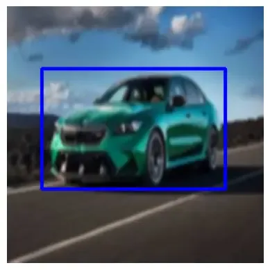
if len(outputs[0]['boxes']) > 0: boxes = outputs[0]['boxes'].detach().numpy() scores = outputs[0]['scores'].detach().numpy() indices = cv2.dnn.NMSBoxes( boxes.tolist(), scores.tolist(), score_threshold=0.5, nms_threshold=0.3) if len(indices) > 0: for i in indices.flatten(): box = boxes[i] cv2.rectangle(img_resized, (int(box[0]), int( box[1])), (int(box[2]), int(box[3])), (255, 0, 0), 2) print("Image processing complete. Visualization requires displaying the image.") import matplotlib.pyplot as plt plt.imshow(cv2.cvtColor(img_resized, cv2.COLOR_BGR2RGB)) plt.axis('off') plt.show() else: print("No objects remaining after NMS.") else: print("No boxes detected by the model.")

Performs non-max suppression to refine detection results, draws bounding boxes on the image and visualizes the final processed image using matplotlib for environments without GUI support.

8. Visualization and Interpretation

Overlay bounding boxes, masks or keypoints on outputs. Display performance metrics including accuracy, precision, recall, F1-score, IoU and confusion matrices. Build interactive and real-time dashboards for monitoring and reporting.

**Overlaying Results: Displaying bounding boxes, segmentation masks and key points on the original images.
**Metrics and Evaluation: Using metrics like accuracy, precision, recall, F1-score and Intersection over Union (IoU) to evaluate model performance.
**User Interface: Developing interactive dashboards or applications to visualize and interpret the results in real-time.

Output:

output

Output