Discrete Fourier Transform (DFT) using Scipy (original) (raw)

Last Updated : 23 Jul, 2025

The Discrete Fourier Transform (DFT) is a powerful mathematical tool used in signal processing, data analysis, image processing and many other fields. It transforms a sequence of values into components of different frequencies revealing the signal's frequency content. In Python DFT is commonly computed using SciPy which provides a simple interface to fast and efficient Fourier transforms.

The DFT converts a finite sequence of equally spaced time domain samples into a sequence of frequency domain components. Mathematically, for a sequence of N complex numbers x0, x1,..., xN-1 the DFT is defined as:

X_k = \sum_{n=0}^{N-1} x_n \cdot e^{-2\pi i kn / N}, \quad \text{for } k = 0, 1, \ldots, N-1

Where,

• X_k: The kth frequency component.
• x_n​: The nth time domain sample.
• N: Total number of samples.
• i: The imaginary unit.
• e^{-2\pi i kn / N}: Complex exponential

Implementation

Step 1: Importing necessary libraries

• numpy is used for numerical operations and creating the time domain signal.
• matplotlib.pyplot is used for plotting the signal and its frequency spectrum.
• **scipy.fft provides: fft: Fast Fourier Transform (computes the DFT), ifft: Inverse FFT (reconstructs time domain signal), fft freq: Computes the frequency bins for plotting. Python `

import numpy as np import matplotlib.pyplot as plt from scipy.fft import fft, ifft, fftfreq

`

Step 2: Create the Time Domain Signal

• fs = 1000 : The signal is sampled at 1000 Hz (1000 samples per second).
• T = 1.0 : Total duration of the signal is 1 second.
• t : A time array of 1000 evenly spaced values between 0 and 1 second (not including 1). Python `

fs = 1000
T = 1.0
t = np.linspace(0, T, int(fs * T), endpoint=False) signal = np.sin(2 * np.pi * 50 * t) + 0.5 * np.sin(2 * np.pi * 120 * t)

`

Step 3: Apply Discrete Fourier Transform (DFT)

• **N = len(t): Number of samples (1000 in this case).
• **fft(signal): Computes the Fast Fourier Transform of the signal converts it from time domain to frequency domain.
• **fftfreq(N, 1/fs): Generates the corresponding frequency values for plotting.
• **np.abs(...): Computes magnitude (amplitude) of complex FFT results.
• **2.0/N: Normalization factor to scale the amplitude correctly. Python `

N = len(t) yf = fft(signal) xf = fftfreq(N, 1/fs)
xf = xf[:N//2] yf = 2.0/N * np.abs(yf[:N//2])

`

Step 4: Plot the Frequency Spectrum

• **plt.figure(figsize=(10, 4)): Sets the size of the plot.
• **plt.plot(xf, yf): Plots amplitude vs. frequency and shows which frequencies are present in the signal.
• Labels and title clarify the graph.
• **plt.grid(True): Adds grid lines for easier reading. Python `

plt.figure(figsize=(10, 4)) plt.plot(xf, yf) plt.title("Frequency Spectrum") plt.xlabel("Frequency (Hz)") plt.ylabel("Amplitude") plt.grid(True) plt.show()

`

**Output:

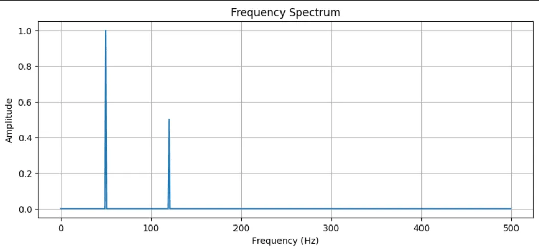
Frequency Spectrum