How to Return the Fit Error in Python curve_fit (original) (raw)
Last Updated : 3 Jul, 2024
The curve fitting method is used in statistics to estimate the output for the best-fit curvy line of a set of data values. Curve fitting is a powerful tool in data analysis that allows us to model the relationship between variables. **In Python, the scipy.optimize.curve_fit function is widely used for this purpose. However, understanding and interpreting the fit errors is crucial for assessing the reliability of the fitted parameters. This article will guide you through the process of returning and interpreting fit errors using curve_fit in Python.
Table of Content
- The curve_fit Function
- Exponential Curve Fitting with curve_fit in Python
- Non-Linear Curve Fitting with curve_fit in Python
The curve_fit Function
Curve fitting involves finding the optimal parameters for a predefined function that best fits a given set of data points. The curve_fit function from the SciPy library uses non-linear least squares to fit a function to the data. The curve_fit function is used to fit a specified model function to a set of data points.
The curve_fit function takes three primary arguments: the function to be fitted (func), the independent variable data (xdata), and the dependent variable data (ydata). **It returns two values: popt (the optimized parameters) and pcov (the covariance matrix of the parameters).
**Here’s a step-by-step outline of how to use it:
- **Import Required Modules: Import the necessary functions and modules, including curve_fit from scipy.optimize, and numpy for numerical operations.
- **Define the Model Function: Create a function that represents the model you want to fit to the data. This function should take the independent variable as the first argument and the parameters to fit as subsequent arguments.
- **Generate or Load Data: Prepare the data points you want to fit. This can be done by generating synthetic data or loading real-world data.
- **Perform the Curve Fit: Use curve_fit to find the optimal parameters for the model function. The function returns the optimal parameters and the covariance matrix.
- **Access Fit Errors: Calculate the standard deviations of the parameters to understand the errors associated with the fit.
Basic Usage of curve_fit: Here's a simple example to illustrate the basic usage of curve_fit:
Python `
import numpy as np from scipy.optimize import curve_fit import matplotlib.pyplot as plt
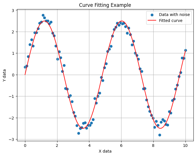
def model_func(x, a, b): return a * np.sin(b * x) np.random.seed(0) xdata = np.linspace(0, 10, 100) y = model_func(xdata, 2.5, 1.3) ydata = y + 0.2 * np.random.normal(size=len(xdata)) plt.figure(figsize=(8, 6)) plt.scatter(xdata, ydata, label='Data with noise')
Fitting the function to the data using curve_fit
popt, pcov = curve_fit(model_func, xdata, ydata)
Getting the optimized parameters
a_opt, b_opt = popt print(f'Optimized parameters: a = {a_opt}, b = {b_opt}') plt.plot(xdata, model_func(xdata, *popt), 'r-', label='Fitted curve')
plt.xlabel('X data') plt.ylabel('Y data') plt.title('Curve Fitting Example') plt.legend() plt.grid(True) plt.show()
`
Output:
Optimized parameters: a = 2.4976290619731176, b = 1.3023626434344653
The curve_fit Function
In this example, curve_fit returns two outputs:
popt: An array of optimal values for the parameters.pcov: The covariance matrix of the parameter estimates.
The diagonal elements of this matrix represent the variance of each parameter. To calculate the standard error (or fit error) of each parameter, we take the square root of the corresponding variance.
Python `
perr = np.sqrt(np.diag(pcov)) perr
`
Output:
array([0.02919289, 0.00188543])
Fit errors are a measure of how well the model is able to explain the data. A small fit error indicates that the parameter is well-constrained by the data, while a large fit error suggests that the parameter is not well-defined. This information is crucial in deciding whether to accept or reject a model.
Exponential Curve Fitting with curve_fit in Python
**Below is a complete example that demonstrates how to use curve_fit and access the fit errors:
Python `
from scipy.optimize import curve_fit import numpy as np import matplotlib.pyplot as plt
Define the model function
def model_func(x, a, b): return a * np.exp(b * x)
Generate some example data
xdata = np.linspace(0, 4, 50) ydata = model_func(xdata, 2.5, 1.3) + 0.2 * np.random.normal(size=len(xdata))
Perform the curve fit
popt, pcov = curve_fit(model_func, xdata, ydata)
Calculate the standard deviations of the parameters
perr = np.sqrt(np.diag(pcov))
Print the results
print("Optimal parameters:", popt) print("Parameter errors:", perr)
Plot the data and the fit
plt.scatter(xdata, ydata, label='Data') plt.plot(xdata, model_func(xdata, *popt), label='Fit', color='red') plt.xlabel('x') plt.ylabel('y') plt.legend() plt.show()
`
**Output:
Optimal parameters: [2.55423726 1.35190947]
Parameter errors: [0.06423982 0.02740202]
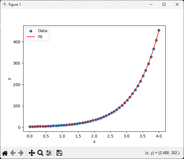
Exponential Curve Fitting with curve_fit in Python
**In this example:
- The model function `model_func` is an exponential function defined as `a * np.exp(b * x)`.
- Synthetic data is generated with some added noise to simulate real-world data.
- `curve_fit` is used to find the optimal parameters `a` and `b` that best fit the data.
- The standard deviations of the parameters, representing the fit errors, are calculated from the covariance matrix.
- The plot visualizes the data points and the fitted curve.
Non-Linear Curve Fitting with curve_fit in Python
Let's consider a more complex example with a non-linear model and real-world data.
Python `
Define a non-linear model function
def non_linear_model(x, a, b, c): return a * np.exp(-b * x) + c x_data = np.linspace(0, 4, 50) y_data = non_linear_model(x_data, 2.5, 1.3, 0.5) + 0.2 * np.random.normal(size=len(x_data)) popt, pcov = curve_fit(non_linear_model, x_data, y_data)
Calculate the standard errors
perr = np.sqrt(np.diag(pcov))
print(f"Optimal parameters: a = {popt[0]}, b = {popt[1]}, c = {popt[2]}") print(f"Standard errors: a_err = {perr[0]}, b_err = {perr[1]}, c_err = {perr[2]}")
Plot the data with error bars
plt.errorbar(x_data, y_data, yerr=0.2, fmt='o', label='Data')
Plot the fitted curve
x_fit = np.linspace(0, 4, 100) y_fit = non_linear_model(x_fit, *popt) plt.plot(x_fit, y_fit, '-', label='Fit')
Add labels and legend
plt.xlabel('x') plt.ylabel('y') plt.legend() plt.show()
`
Output:
Optimal parameters: a = 2.498240343789229, b = 1.1235023885202289, c = 0.48110201669612906
Standard errors: a_err = 0.11746465918381212, b_err = 0.12517346932091297, c_err = 0.06317613094514635
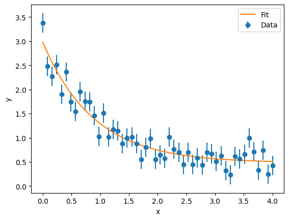
Non-Linear Curve Fitting with curve_fit in Python
Conclusion
Understanding and interpreting fit errors is crucial for assessing the reliability of fitted parameters in curve fitting. The scipy.optimize.curve_fit function provides a powerful tool for fitting data to models, and the covariance matrix it returns allows us to quantify the uncertainties of the fitted parameters. By extracting the standard errors and calculating confidence intervals, we can gain valuable insights into the precision and reliability of our model.