Quadratic Discriminant Analysis (original) (raw)
Last Updated : 7 Jan, 2022
Linear Discriminant Analysis
Now, Let's consider a classification problem represented by a Bayes Probability distribution P(Y=k | X=x), LDA does it differently by trying to model the distribution of X given the predictors class (I.e. the value of Y) P(X=x| Y=k):
P(Y=k | X=x) = \frac{P(X=x | Y=k) P(Y=k)}{P(X=x)}
= \frac{P(X=x | Y=k) P(Y=k)}{\sum_{j=1}^{K} P(X=x | Y=j) P(Y=j)}
In LDA, we assume that P(X | Y=k) can be estimated to the multivariate Normal distribution that is given by following equation:
f_k(x) = \frac{1}{(2\pi)^{p/2}|\mathbf\Sigma|^{1/2}} e^{-\frac{1}{2}(x-\mu_k)^T \mathbf{\Sigma}^{-1}(x-\mu_k)}
where, \mu_k = mean\, of\, the\, examples\, of \, category\, k \\ \mathbf{\sum} = covariance \, (we\, assume\, common\, covariance\, for\, all\, categories)
and P(Y=k) =\pi_k. Now, we try to write the above equation with the assumptions:
P(Y=k | X=x) = \frac{\pi_k \frac{1}{(2\pi)^{p/2}|\mathbf\Sigma|^{1/2}} e^{-\frac{1}{2}(x-\mu_k)^T \mathbf{\Sigma}^{-1}(x-\mu_k)}}{\sum_{j=1}^{K} \frac{1}{(2\pi)^{p/2}|\mathbf\Sigma|^{1/2}} e^{-\frac{1}{2}(x-\mu_j)^T \mathbf{\Sigma}^{-1}(x-\mu_j)}}
Now, we take log both sides and maximizing the equation, we get the decision boundary:
\delta_k(x) = \log \pi_k - \frac{1}{2}\mu_k^T \Sigma^{-1}\mu_k + x^T \Sigma^{-1}\mu_k
For two classes, the decision boundary is a linear function of x where both classes give equal value, this linear function is given as:
\left\{x: \delta_k(x) = \delta_{\ell}(x) \right\}, 1 \leq j,\ell \leq K
For multi-class (K>2), we need to estimate the pK means, pK variance, K prior proportions and \binom{p}{2}K = \left ( \frac{p(p-1)}{2} \right )K . Now, we discuss in more detail about Quadratic Discriminant Analysis.
Quadratic Discriminant Analysis
Quadratic discriminant analysis is quite similar to Linear discriminant analysis except we relaxed the assumption that the mean and covariance of all the classes were equal. Therefore, we required to calculate it separately.
Now, for each of the class y the covariance matrix is given by:
\Sigma_y = \frac{1}{N_y-1} \sum_{y_i = y} (x_i - \mu_y)(x_i -\mu_y)^T
By adding the following term and solving (taking log both side and ). The quadratic Discriminant function is given by:
\delta_k(x) = \log \pi_k - \frac{1}{2}\mu_k^T \mathbf{\Sigma}_k^{-1}\mu_k + x^T \mathbf{\Sigma}_k^{-1}\mu_k - \frac{1}{2}x^T \Sigma_k^{-1}x -\frac{1}{2}\log |\Sigma_k|
Implementation
- In this implementation, we will be using R and MASS library to plot the decision boundary of Linear Discriminant Analysis and Quadratic Discriminant Analysis. For this, we will use iris dataset: R `
import libraries
library(caret) library(MASS) library(tidyverse)
Code to plot decision plot
decision_boundary = function(model, data,vars, resolution = 200,...) { class='Species' labels_var = data[,class] k = length(unique(labels_var))
For sepals
if (vars == 'sepal'){ data = data %>% select(Sepal.Length, Sepal.Width) } else{ data = data %>% select(Petal.Length, Petal.Width) }
plot with color labels
int_labels = as.integer(labels_var) plot(data, col = int_labels+1L, pch = int_labels+1L, ...)
make grid
r = sapply(data, range, na.rm = TRUE) xs = seq(r[1,1], r[2,1], length.out = resolution) ys = seq(r[1,2], r[2,2], length.out = resolution) dfs = cbind(rep(xs, each=resolution), rep(ys, time = resolution))
colnames(dfs) = colnames(r) dfs = as.data.frame(dfs)
p = predict(model, dfs, type ='class' ) p = as.factor(p$class)
points(dfs, col = as.integer(p)+1L, pch = ".")
mats = matrix(as.integer(p), nrow = resolution, byrow = TRUE) contour(xs, ys, mats, add = TRUE, lwd = 2, levels = (1:(k-1))+.5)
invisible(mats) }
par(mfrow=c(2,2))
run the linear discriminant analysis and plot the decision boundary with Sepals variable
model = lda(Species ~ Sepal.Length + Sepal.Width, data=iris) lda_sepals = decision_boundary(model, iris, vars= 'sepal' , main = "LDA_Sepals")
run the quadratic discriminant analysis and plot the decision boundary with Sepals variable
model_qda = qda(Species ~ Sepal.Length + Sepal.Width, data=iris) qda_sepals = decision_boundary(model_qda, iris, vars= 'sepal', main = "QDA_Sepals")
run the linear discriminant analysis and plot the decision boundary with Petals variable
model = lda(Species ~ Petal.Length + Petal.Width, data=iris) lda_petal =decision_boundary(model, iris, vars='petal', main = "LDA_petals")
run the quadratic discriminant analysis and plot the decision boundary with Petals variable
model_qda = qda(Species ~ Petal.Length + Petal.Width, data=iris) qda_petal =decision_boundary(model_qda, iris, vars='petal', main = "QDA_petals")
`
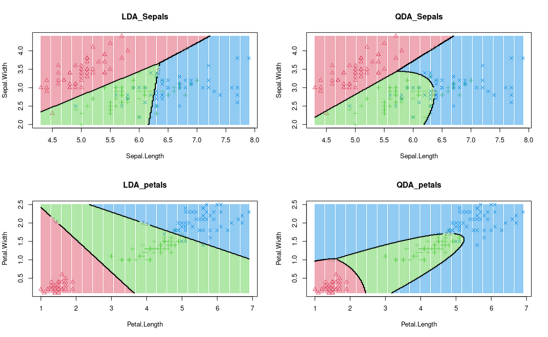
LDA and QDA visualization