Ordinary Least Squares (OLS) using statsmodels (original) (raw)

Last Updated : 15 Jul, 2025

Ordinary Least Squares (OLS) is a widely used statistical method for estimating the parameters of a linear regression model. It minimizes the sum of squared residuals between observed and predicted values. In this article we will learn how to implement **Ordinary Least Squares (OLS) regression using Python's statsmodels module.

Overview of Linear Regression Model

A **linear regression model establishes the relationship between a dependent variable (_y) and one or more independent variables (_x):

\hat{y} = b_1 x + b_0

Where:

• \hat{y} : Predicted value of _y
• __b_1​: Slope of the line (coefficient of _x)
• __b_0​: Intercept (value of _y when __x_=0)

The **OLS method minimizes the total sum of squares of residuals (_S) defined as:

S = \sum_{i=1}^{n} \epsilon_i^2 = \sum_{i=1}^{n} (y_i - \hat{y}_i)^2

To find the optimal values of __b_0​ and __b_1​ partial derivatives of _S with respect to each coefficient are taken and set to zero.

**Implementation OLS Regression Using Statsmodels

**Step 1: Import Required Libraries

Before starting, we need to import necessary libraries like pandas , numpy and matplotlib.

Python `

import statsmodels.api as sm import pandas as pd
import matplotlib.pyplot as plt import numpy as np

`

**Step 2: Load and Prepare the Data

We load the dataset from a CSV file using pandas. You can download dataset from here. The dataset contains two columns:

• x: Independent variable (predictor).
• y: Dependent variable (response). Python `

data = pd.read_csv('train.csv')

x = data['x'].tolist()
y = data['y'].tolist()

`

**Step 3: Add a Constant Term

In linear regression the equation includes an intercept term (__b_0​). To include this term in the model we use the add_constant() function from statsmodels.

Python `

x = sm.add_constant(x)

`

**Step 4: Perform OLS Regression

Now we fit the OLS regression model using the OLS() function. This function takes the dependent variable (_y) and the independent variable (_x) as inputs.

Python `

result = sm.OLS(y, x).fit()

print(result.summary())

`

**Output :

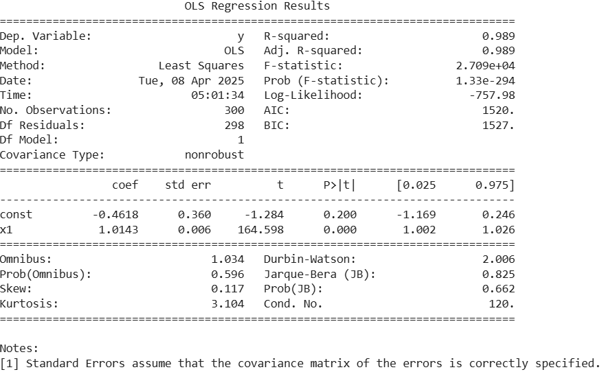
• The output shows that the regression model fits the data very well with an R-squared of 0.989.
• The independent variable x1 is highly significant (p < 0.001) and has a strong positive effect on the target variable.
• The intercept (const) is not statistically significant (p = 0.200) meaning it may not contribute meaningfully.
• Residuals are normally distributed as indicated by the Omnibus and Jarque-Bera test p-values (> 0.05).
• The Durbin-Watson value is ~2 indicating no autocorrelation in residuals.
• The overall model is statistically significant with a very high F-statistic and a near-zero p-value

**Step 5: Visualize the Regression Line

To better understand the relationship between _x and _y we plot the original data points and the fitted regression line.

Python `

plt.scatter(data['x'], data['y'], color='blue', label='Data Points')

x_range = np.linspace(data['x'].min(), data['x'].max(), 100) y_pred = result.params[0] + result.params[1] * x_range

plt.plot(x_range, y_pred, color='red', label='Regression Line') plt.xlabel('Independent Variable (X)') plt.ylabel('Dependent Variable (Y)') plt.title('OLS Regression Fit') plt.legend() plt.show()

`

**Output:

Regression Line

The above plot shows a strong linear relationship between the independent variable (X) and the dependent variable (Y). Blue dots represent the actual data points which are closely aligned with the red regression line indicating a good model fit.