Applying Convolutional Neural Network on mnist dataset (original) (raw)
Last Updated : 12 Aug, 2024
**CNN is a model known to be a **Convolutional Neural Network and in recent times it has gained a lot of popularity because of its usefulness. CNN uses multilayer perceptrons to do computational work. CNN uses relatively little pre-processing compared to other image classification algorithms. This means the network learns through filters that in traditional algorithms were hand-engineered. So, for the image processing tasks, CNNs are the best-suited option.
Applying a Convolutional Neural Network (CNN) on the MNIST dataset is a popular way to learn about and demonstrate the capabilities of CNNs for image classification tasks. The MNIST dataset consists of 28x28 grayscale images of hand-written digits (0-9), with a training set of 60,000 examples and a test set of 10,000 examples.
Here is a basic approach to applying a CNN on the MNIST dataset using the Python programming language and the Keras library:
- Load and preprocess the data: The MNIST dataset can be loaded using the Keras library, and the images can be normalized to have pixel values between 0 and 1.
- Define the model architecture: The CNN can be constructed using the Keras Sequential API, which allows for easy building of sequential models layer-by-layer. The architecture should typically include convolutional layers, pooling layers, and fully-connected layers.
- Compile the model: The model needs to be compiled with a loss function, an optimizer, and a metric for evaluation.
- Train the model: The model can be trained on the training set using the Keras fit() function. It is important to monitor the training accuracy and loss to ensure the model is converging properly.
- Evaluate the model: The trained model can be evaluated on the test set using the Keras evaluate() function. The evaluation metric typically used for classification tasks is accuracy.
Here are some tips and best practices to keep in mind when applying a CNN on the MNIST dataset:
- Start with a simple architecture and gradually increase complexity if necessary.
- Experiment with different activation functions, optimizers, learning rates, and batch sizes to find the optimal combination for your specific task.
- Use regularization techniques such as dropout or weight decay to prevent overfitting.
- Visualize the filters and feature maps learned by the model to gain insights into its inner workings.
- Compare the performance of the CNN to other machine learning algorithms such as Support Vector Machines or Random Forests to get a sense of its relative performance.
References:
- MNIST dataset: http://yann.lecun.com/exdb/mnist/
- Keras documentation: https://keras.io/
- "Deep Learning with Python" by Francois Chollet (https://www.manning.com/books/deep-learning-with-python)
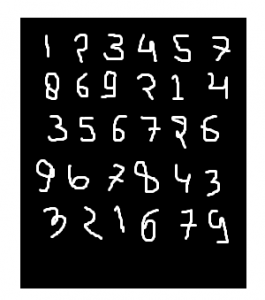
**MNIST dataset:
mnist dataset is a dataset of handwritten images as shown below in the image.
We can get 99.06% accuracy by using CNN(Convolutional Neural Network) with a functional model. The reason for using a functional model is to maintain easiness while connecting the layers.
Firstly, include all necessary libraries
Python3 `
import numpy as np import keras from keras.datasets import mnist from keras.models import Model from keras.layers import Dense, Input from keras.layers import Conv2D, MaxPooling2D, Dropout, Flatten from keras import backend as k
`
Create the train data and test data
- **Test data: Used for testing the model that how our model has been trained.
**Train data: Used to train our model. Python3 `
(x_train, y_train), (x_test, y_test) = mnist.load_data()
`
- While proceeding further, **img_rows and **img_cols are used as the image dimensions. In mnist dataset, it is 28 and 28. We also need to check the data format i.e. 'channels_first' or 'channels_last'. In CNN, we can normalize data before hands such that large terms of the calculations can be reduced to smaller terms. Like, we can normalize the x_train and x_test data by dividing it by 255.
**Checking data-format: Python3 `
img_rows, img_cols=28, 28
if k.image_data_format() == 'channels_first': x_train = x_train.reshape(x_train.shape[0], 1, img_rows, img_cols) x_test = x_test.reshape(x_test.shape[0], 1, img_rows, img_cols) inpx = (1, img_rows, img_cols)
else: x_train = x_train.reshape(x_train.shape[0], img_rows, img_cols, 1) x_test = x_test.reshape(x_test.shape[0], img_rows, img_cols, 1) inpx = (img_rows, img_cols, 1)
x_train = x_train.astype('float32') x_test = x_test.astype('float32') x_train /= 255 x_test /= 255
`
Description of the output classes:
- Since the output of the model can comprise any of the digits between 0 to 9. so, we need 10 classes in output. To make output for 10 classes, use keras.utils.to_categorical function, which will provide the 10 columns. Out of these 10 columns, only one value will be one and the rest 9 will be zero and this one value of the output will denote the class of the digit. Python3 `
y_train = keras.utils.to_categorical(y_train) y_test = keras.utils.to_categorical(y_test)
`
- Now, the dataset is ready so let's move towards the CNN model : Python3 `
inpx = Input(shape=inpx) layer1 = Conv2D(32, kernel_size=(3, 3), activation='relu')(inpx) layer2 = Conv2D(64, (3, 3), activation='relu')(layer1) layer3 = MaxPooling2D(pool_size=(3, 3))(layer2) layer4 = Dropout(0.5)(layer3) layer5 = Flatten()(layer4) layer6 = Dense(250, activation='sigmoid')(layer5) layer7 = Dense(10, activation='softmax')(layer6)
`
- **Explanation of the working of each layer in the **CNN model:
layer1 is the Conv2d layer which convolves the image using 32 filters each of size (3*3).
layer2 is again a Conv2D layer which is also used to convolve the image and is using 64 filters each of size (3*3).
layer3 is the MaxPooling2D layer which picks the max value out of a matrix of size (3*3).
layer4 is showing Dropout at a rate of 0.5.
layer5 is flattening the output obtained from layer4 and this flattens output is passed to layer6.
layer6 is a hidden layer of a neural network containing 250 neurons.
layer7 is the output layer having 10 neurons for 10 classes of output that is using the softmax function. - **Calling compile and fit function: Python3 `
model = Model([inpx], layer7) model.compile(optimizer=keras.optimizers.Adadelta(), loss=keras.losses.categorical_crossentropy, metrics=['accuracy'])
model.fit(x_train, y_train, epochs=12, batch_size=500)
`
**Output:
Epoch 1/12
120/120 ━━━━━━━━━━━━━━━━━━━━ 154s 1s/step - accuracy: 0.0968 - loss: 2.4955
Epoch 2/12
120/120 ━━━━━━━━━━━━━━━━━━━━ 201s 1s/step - accuracy: 0.0957 - loss: 2.4752
Epoch 3/12
120/120 ━━━━━━━━━━━━━━━━━━━━ 203s 1s/step - accuracy: 0.0995 - loss: 2.4479
Epoch 4/12
120/120 ━━━━━━━━━━━━━━━━━━━━ 151s 1s/step - accuracy: 0.0984 - loss: 2.4262
Epoch 5/12
120/120 ━━━━━━━━━━━━━━━━━━━━ 204s 1s/step - accuracy: 0.0980 - loss: 2.4085
Epoch 6/12
120/120 ━━━━━━━━━━━━━━━━━━━━ 201s 1s/step - accuracy: 0.0970 - loss: 2.3864
Epoch 7/12
120/120 ━━━━━━━━━━━━━━━━━━━━ 202s 1s/step - accuracy: 0.0982 - loss: 2.3699
Epoch 8/12
120/120 ━━━━━━━━━━━━━━━━━━━━ 152s 1s/step - accuracy: 0.0972 - loss: 2.3520
Epoch 9/12
120/120 ━━━━━━━━━━━━━━━━━━━━ 201s 1s/step - accuracy: 0.0975 - loss: 2.3324
Epoch 10/12
120/120 ━━━━━━━━━━━━━━━━━━━━ 203s 1s/step - accuracy: 0.0966 - loss: 2.3151
Epoch 11/12
120/120 ━━━━━━━━━━━━━━━━━━━━ 153s 1s/step - accuracy: 0.0960 - loss: 2.3017
Epoch 12/12
120/120 ━━━━━━━━━━━━━━━━━━━━ 201s 1s/step - accuracy: 0.0972 - loss: 2.2847
<keras.src.callbacks.history.History at 0x7b04c491e200>
- Firstly, we made an object of the model as shown in the above-given lines, where [inpx] is the input in the model and layer7 is the output of the model. We compiled the model using the required optimizer, loss function and printed the accuracy and at the last model.fit was called along with parameters like x_train(means image vectors), y_train(means the label), number of epochs, and the batch size. Using fit function x_train, y_train dataset is fed to model in particular batch size.
- **Evaluate function:
model.evaluate provides the score for the test data i.e. provided the test data to the model. Now, the model will predict the class of the data, and the predicted class will be matched with the y_test label to give us the accuracy. Python3 `
score = model.evaluate(x_test, y_test, verbose=0) print('loss=', score[0]) print('accuracy=', score[1])
`
**Output:
loss= 2.269895553588867
accuracy= 0.09950000047683716