Conditional Generative Adversarial Network (original) (raw)

Last Updated : 18 May, 2026

Conditional Generative Adversarial Networks (CGANs) are a type of GAN that generate data based on specific conditions such as labels or descriptions. Unlike standard GANs that produce random outputs, CGANs use additional information to control the generation process and create more targeted results.

Generates data based on given conditions or labels
Produces more controlled and precise outputs than standard GANs
Uses conditional information in both generator and discriminator
Can generate category-specific images or data

Architecture and Working

Conditional GANs (CGANs) extend traditional GANs by conditioning both the generator and discriminator on additional information such as labels or descriptions. This conditioning makes the generation process more controlled and targeted.

1. Generator in CGANs

The generator creates synthetic data such as images, text, or videos using two inputs

**Inputs

**Random Noise (z): A vector of random values that adds diversity to generated outputs.
**Conditioning Information (y): Extra data like labels or context that guides what the generator produces for example a class label such as "cat" or "dog".

**Working: The generator combines z and y to create realistic data matching the given condition.

**Example: If the condition is “cat”, the generator produces an image of a cat.

2. Discriminator in CGANs

The discriminator determines whether the input data is real or generated while also checking if it matches the given condition.

**Inputs

**Real Data (x): Actual samples from the dataset.
**Conditioning Information (y): The same condition given to the generator.

**Working: The discriminator learns to verify both

Whether the data is real or fake
Whether it correctly matches the condition

**Example: If an image is labeled “cat”, the discriminator checks whether it genuinely looks like a cat.

3. Interaction Between Generator and Discriminator

The generator and discriminator train together in a competitive process.

**Generator Goal: Generate fake data that appears real to the discriminator
**Discriminator Goal: Correctly distinguish between real and fake data using the condition

4. Loss Function and Training

The training process is guided by the adversarial loss function

min_G max_D V(D,G) = \mathbb{E}_{x \sim p_{data} (x)}[logD(x|y)] + \mathbb{E}_{z \sim p_{z}}(z)[log(1- D(G(z∣y)))]

The first term encourages the discriminator to classify real samples correctly.
The second term pushes the generator to produce samples that the discriminator classifies as real.

Here \mathbb{E} represents the expected value p_{data} is the real data distribution and p_{z} is the prior noise distribution.

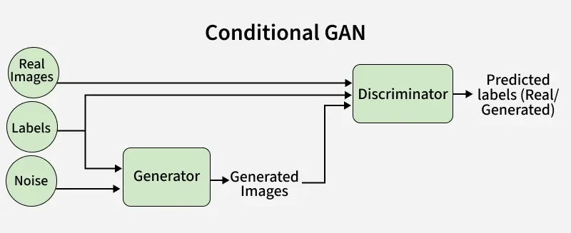
conditional_gan

Conditional GAN

Implementation

We will build and train a Conditional Generative Adversarial Network (CGAN) to generate class-specific images from the CIFAR-10 dataset. Below are the key steps involved:

Step 1: Importing Necessary Libraries

We will import TensorFlow, NumPy, Keras and Matplotlib libraries for building models, loading data and visualization.

Python `

import tensorflow as tf from tensorflow.keras.models import Model from tensorflow.keras.optimizers import Adam from tensorflow.keras.datasets import cifar10 from keras.preprocessing import image import keras.backend as K import matplotlib.pyplot as plt import numpy as np import time from tqdm import tqdm

Step 2: Loading Dataset and Declaring Variables

Load the CIFAR-10 dataset using TensorFlow datasets or tf.data.Dataset.
Define global variables such as number of epochs, batch size and image dimensions. Python `

batch_size = 16 epoch_count = 50 noise_dim = 100 n_class = 10 tags = ['Airplane', 'Automobile', 'Bird', 'Cat', 'Deer', 'Dog', 'Frog', 'Horse', 'Ship', 'Truck'] img_size = 32

(X_train, y_train), (_, _) = cifar10.load_data()

X_train = (X_train - 127.5) / 127.5

dataset = tf.data.Dataset.from_tensor_slices((X_train, y_train)) dataset = dataset.shuffle(buffer_size=1000).batch(batch_size)

cgans1

Downloading data

Step 3: Visualizing Sample Images

Now we will visualize the images from the dataset to understand class distributions and data shape.

Python `

plt.figure(figsize=(2,2)) idx = np.random.randint(0,len(X_train)) img = image.array_to_img(X_train[idx], scale=True) plt.imshow(img) plt.axis('off') plt.title(tags[y_train[idx][0]]) plt.show()

**Output:

cgans2

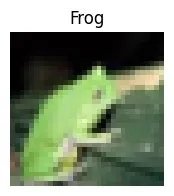
Sample Image

Step 4: Defining Loss Functions and Optimizers

In the next step we need to define the Loss function and optimizer for the discriminator and generator networks in a Conditional Generative Adversarial Network(CGANS).

Use Binary Cross-Entropy Loss for both generator and discriminator.
Define discriminator loss as sum of real and fake losses.
The binary entropy calculates two losses: real_loss: Loss when the discriminator tries to classify real data as real and fake_loss : Loss when the discriminator tries to classify fake data as fake
d_optimizer and g_optimizer are used to update the trainable parameters of the discriminator and generator during training.
Use Adam optimizer for both networks. Python `

bce_loss = tf.keras.losses.BinaryCrossentropy()

def discriminator_loss(real, fake): real_loss = bce_loss(tf.ones_like(real), real) fake_loss = bce_loss(tf.zeros_like(fake), fake) total_loss = real_loss + fake_loss return total_loss

def generator_loss(preds): return bce_loss(tf.ones_like(preds), preds)

d_optimizer=Adam(learning_rate=0.0002, beta_1 = 0.5) g_optimizer=Adam(learning_rate=0.0002, beta_1 = 0.5)

Step 5: Building the Generator Model

Input is noise vector (latent space) and label.
Convert label to a vector using an embedding layer (size 50).
Process noise through dense layers with LeakyReLU activation.
Reshape and concatenate label embedding with noise features.
Use Conv2DTranspose layers to up-sample into 32×32×3 images.
Output layer uses tanh activation to scale pixels between -1 and 1. Python `

def build_generator():

in_label = tf.keras.layers.Input(shape=(1,))
li = tf.keras.layers.Embedding(n_class, 50)(in_label)

n_nodes = 8 * 8
li = tf.keras.layers.Dense(n_nodes)(li)
li = tf.keras.layers.Reshape((8, 8, 1))(li)
in_lat = tf.keras.layers.Input(shape=(noise_dim,))

n_nodes = 128 * 8 * 8
gen = tf.keras.layers.Dense(n_nodes)(in_lat)
gen = tf.keras.layers.LeakyReLU(alpha=0.2)(gen)
gen = tf.keras.layers.Reshape((8, 8, 128))(gen)
merge = tf.keras.layers.Concatenate()([gen, li])

gen = tf.keras.layers.Conv2DTranspose(
    128, (4, 4), strides=(2, 2), padding='same')(merge)  
gen = tf.keras.layers.LeakyReLU(alpha=0.2)(gen)

gen = tf.keras.layers.Conv2DTranspose(
    128, (4, 4), strides=(2, 2), padding='same')(gen)  
gen = tf.keras.layers.LeakyReLU(alpha=0.2)(gen)

out_layer = tf.keras.layers.Conv2D(
    3, (8, 8), activation='tanh', padding='same')(gen)  

model = Model([in_lat, in_label], out_layer)
return model

g_model = build_generator() g_model.summary()

**Output:

cgans3

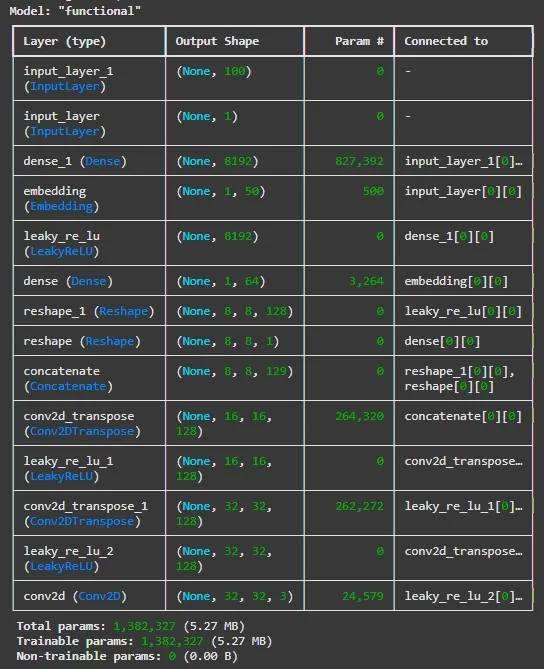
Building the Generator Model

Step 6: Building the Discriminator Model

Input is our image and label.
Embed label into a 50-dimensional vector.
Reshape and concatenate label embedding with the input image.
Apply two Conv2D layers with LeakyReLU activations to extract features.
Flatten features, apply dropout to prevent overfitting.
Final dense layer with sigmoid activation outputs probability of real or fake. Python `

def build_discriminator():

in_label = tf.keras.layers.Input(shape=(1,))

li = tf.keras.layers.Embedding(n_class, 50)(in_label)

n_nodes = img_size * img_size li = tf.keras.layers.Dense(n_nodes)(li)

li = tf.keras.layers.Reshape((img_size, img_size, 1))(li)

in_image = tf.keras.layers.Input(shape=(img_size, img_size, 3))

merge = tf.keras.layers.Concatenate()([in_image, li])

fe = tf.keras.layers.Conv2D(128, (3,3), strides=(2,2), padding='same')(merge) fe = tf.keras.layers.LeakyReLU(alpha=0.2)(fe)

fe = tf.keras.layers.Conv2D(128, (3,3), strides=(2,2), padding='same')(fe) fe = tf.keras.layers.LeakyReLU(alpha=0.2)(fe)

fe = tf.keras.layers.Flatten()(fe)

fe = tf.keras.layers.Dropout(0.4)(fe)

out_layer = tf.keras.layers.Dense(1, activation='sigmoid')(fe)

model = Model([in_image, in_label], out_layer)

return model d_model = build_discriminator() d_model.summary()

**Output:

cgans4

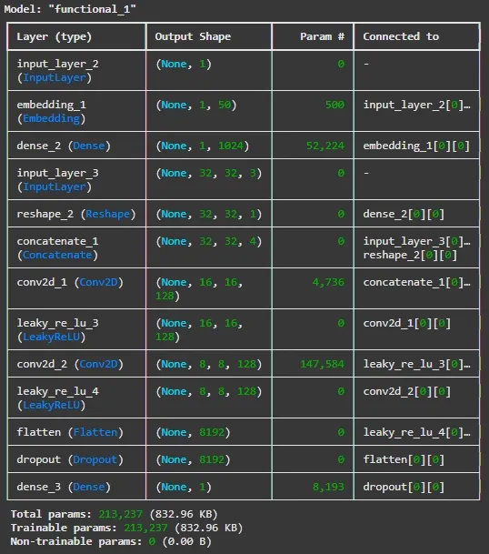
Building the Discriminator Model

Step 7: Creating Training Step Function

Use TensorFlow’s Gradient Tape to calculate and apply gradients for both networks.
Alternate training discriminator on real and fake data.
Train generator to fool discriminator.
Use @tf.function for efficient graph execution. Python `

@tf.function def train_step(dataset):

real_images, real_labels = dataset

random_latent_vectors = tf.random.normal(shape=(batch_size, noise_dim))
generated_images = g_model([random_latent_vectors, real_labels])

with tf.GradientTape() as tape:
    pred_fake = d_model([generated_images, real_labels])
    pred_real = d_model([real_images, real_labels])
    
    d_loss = discriminator_loss(pred_real, pred_fake)
  
grads = tape.gradient(d_loss, d_model.trainable_variables)

d_optimizer.apply_gradients(zip(grads, d_model.trainable_variables))


random_latent_vectors = tf.random.normal(shape=(batch_size, noise_dim))


with tf.GradientTape() as tape:
    fake_images = g_model([random_latent_vectors, real_labels])
    predictions = d_model([fake_images, real_labels])
    g_loss = generator_loss(predictions)

grads = tape.gradient(g_loss, g_model.trainable_variables)
g_optimizer.apply_gradients(zip(grads, g_model.trainable_variables))

return d_loss, g_loss

Step 8: Visualizing Generated Images

After each epoch we will generate images conditioned on different labels.
Display or save generated images to monitor training progress. Python `

def show_samples(num_samples, n_class, g_model): fig, axes = plt.subplots(10,num_samples, figsize=(10,20)) fig.tight_layout() fig.subplots_adjust(wspace=None, hspace=0.2)

for l in np.arange(10):
  random_noise = tf.random.normal(shape=(num_samples, noise_dim))
  label = tf.ones(num_samples)*l
  gen_imgs = g_model.predict([random_noise, label])
  for j in range(gen_imgs.shape[0]):
    img = image.array_to_img(gen_imgs[j], scale=True)
    axes[l,j].imshow(img)
    axes[l,j].yaxis.set_ticks([])
    axes[l,j].xaxis.set_ticks([])

    if j ==0:
      axes[l,j].set_ylabel(tags[l])
plt.show()

Step 9: Train the Model

At the final step we will start training the model for specified epochs.
Print losses regularly to monitor performance.
Longer training typically results in higher quality images. Python `

def train(dataset, epochs=epoch_count):

for epoch in range(epochs):
    print('Epoch: ', epochs)
    d_loss_list = []
    g_loss_list = []
    q_loss_list = []
    start = time.time()
    
    itern = 0
    for image_batch in tqdm(dataset):
        d_loss, g_loss = train_step(image_batch)
        d_loss_list.append(d_loss)
        g_loss_list.append(g_loss)
        itern=itern+1
            
    show_samples(3, n_class, g_model)
        
    print (f'Epoch: {epoch} -- Generator Loss: {np.mean(g_loss_list)}, Discriminator Loss: {np.mean(d_loss_list)}\n')
    print (f'Took {time.time()-start} seconds. \n\n')

train(dataset, epochs=epoch_count)

**Output:

cgans5

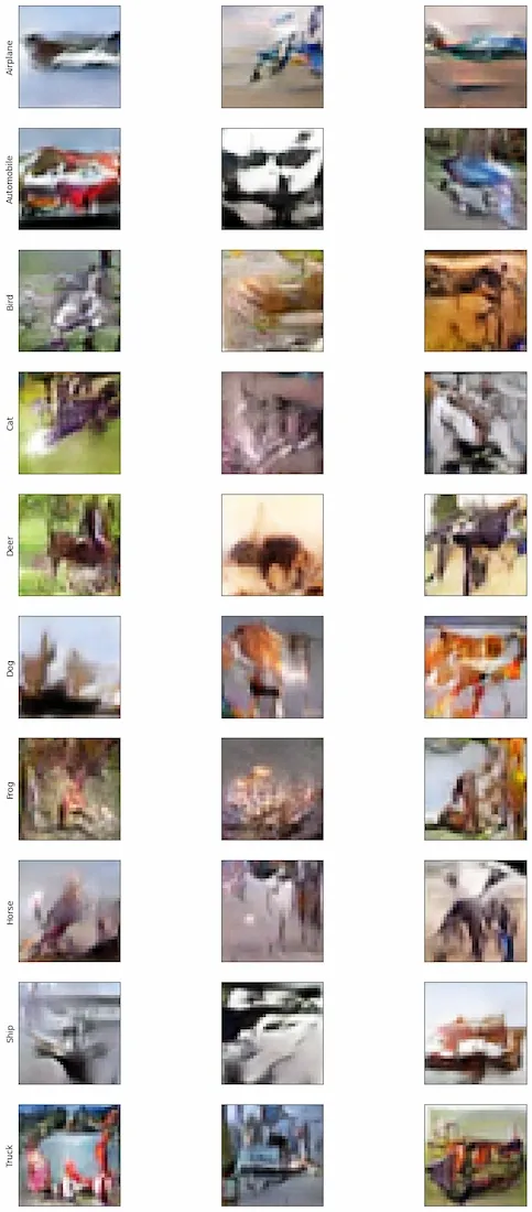
Output Images

We can see some details in these pictures. But for better result we can try to run this for more epochs.

Download full code from here