Generative Adversarial Networks (GANs) with R (original) (raw)
Last Updated : 30 Apr, 2026
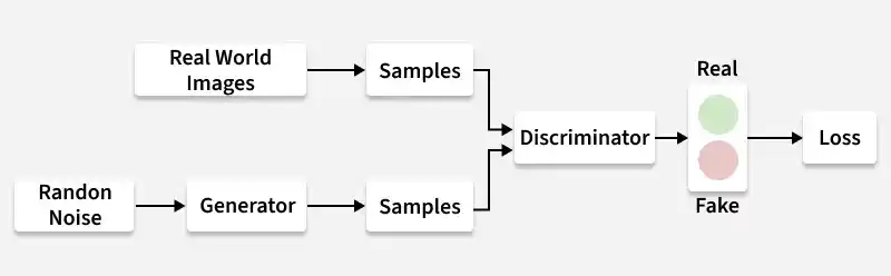
Generative Adversarial Networks (GANs) are deep learning models used to generate realistic synthetic data by learning patterns from real datasets. They are widely applied in tasks such as image generation, video synthesis and data augmentation.
GANs consist of two neural networks that compete with each other during training:
- **Generator: The generator creates new synthetic data from random noise. Its goal is to produce data that looks as realistic as possible so that it becomes difficult to distinguish from real data.
- **Discriminator: The discriminator evaluates the data and determines whether it is real (from the dataset) or fake (generated by the generator). Its feedback helps the generator improve and produce more realistic outputs over time.
Working
Generative Adversarial Networks (GANs) use two neural networks called the Generator (G) and the Discriminator (D) that compete with each other during training. Both networks are trained together in a competitive process, known as adversarial training, where the generator improves its ability to create realistic data and the discriminator improves its ability to detect fake samples.
1. Generator Model
The Generator is a deep neural network responsible for generating synthetic data samples. It takes a random noise vector as input and transforms it into data that resembles real examples from the training dataset.
- During training, the generator learns the underlying patterns of the dataset by adjusting its parameters.
- The parameters are updated using the backpropagation algorithm.
- The main objective of the generator is to produce realistic synthetic samples.
- These generated samples should be convincing enough to fool the discriminator into classifying them as real data.
The generator tries to minimize the adversarial loss:
J_G = -\frac{1}{m} \sum_{i=1}^{m} \log D(G(z_i))
where
- J_{G} represents the generator loss.
- z_{i} is a random noise vector.
- G(Z_{i}) is the generated sample.
- D(G(z_{i})) is the probability estimated by the discriminator that the generated sample is real.
- m represents the number of samples in a batch.
2. Discriminator Model
The Discriminator is a neural network that acts as a binary classifier. Its role is to determine whether a given sample comes from the real dataset or is generated by the generator. The discriminator receives two types of inputs:
- Real data samples from the training dataset
- Fake data samples generated by the generator
The discriminator outputs a probability between 0 and 1, where 1 indicates the data is likely real and 0 indicates it is likely fake.
For image-related tasks, the discriminator often uses convolutional neural networks (CNNs) to extract features and improve classification accuracy.
**Discriminator Loss Function
The objective of the discriminator is to minimize the loss:
J_D = -\frac{1}{m} \sum_{i=1}^{m} \log D(x_i) - \frac{1}{m} \sum_{i=1}^{m} \log(1 - D(G(z_i)))
where
- J_{D} represents the discriminator loss.
- G(Z_{i}) is a generated (fake) sample.
- D(x_{i}) is the probability that the real sample is classified as real.
The discriminator aims to:
- Maximize log D(x_{i}) so that real samples are classified correctly.
- Maximize log(1-D(G(z_{i}))) so that fake samples are correctly identified.
3. Min–Max Objective Function
GANs are trained using a min–max optimization objective, where the generator tries to minimize the objective while the discriminator tries to maximize it.
- The generator tries to minimize the loss to fool the discriminator.
- The discriminator tries to maximize the loss to correctly detect fake samples.
\min_{G} \max_{D} V(G, D) = E_{x \sim p_{data}(x)}[\log D(x)] + E_{z \sim p_{z}(z)}[\log(1 - D(G(z)))]
where
- G represents the generator network
- D represents the discriminator network
- p_{data}(x) represents the true data distribution
- p_{z}(z) represents the random noise distribution
Training Process of GANs
The training of GANs involves an iterative process where both networks continuously improve by competing against each other.
GAN Traning Process
**Step 1: Generator Creates Fake Data
The generator starts with a random noise vector as input. Using its neural network layers, it transforms this noise into a synthetic data sample such as an image.
**Step 2: Discriminator Receives Real and Fake Data
The discriminator is given two types of inputs:
- Real data from the dataset
- Fake data produced by the generator
It evaluates each sample and outputs a probability indicating whether the sample is real or fake.
**Step 3: Discriminator Training
The discriminator calculates its loss by comparing its predictions with the true labels:
- Real data should be labeled 1
- Generated data should be labeled 0
Using backpropagation, the discriminator updates its weights to improve its ability to distinguish between real and fake samples.
**Step 4: Generator Training
Generator is trained using the feedback from the discriminator. The generator attempts to produce data that causes the discriminator to classify it as real. The generator updates its parameters based on the discriminator's feedback to generate more realistic samples.
**Step 5: Adversarial Learning
This process creates a competition between the generator and discriminator:
- The generator improves its ability to create realistic data.
- The discriminator improves its ability to detect fake data.
Step 6: Training Convergence
After many training iterations:
- The generator becomes highly skilled at producing realistic samples.
- The discriminator finds it increasingly difficult to distinguish real data from generated data.
At this stage, the generator can produce high-quality synthetic data that closely resembles real-world data.
Step By Step Implementation
Here we implement GAN in R programming language.
Step 1: Install and Load Required Libraries
Install and load the required R libraries. These libraries help build and train deep learning models using Keras and TensorFlow in R.
R `
install.packages("keras") install.packages("tensorflow") install.packages("abind")
library(keras) library(tensorflow) library(abind)
`
Step 2: Load the MNIST Dataset
Here we load the MNIST dataset, which contains handwritten digit images. We then extract the training and test data that will be used for building and evaluating the GAN model.
R `
Load the MNIST dataset
mnist <- dataset_mnist()
Extract training and test data
x_train <- mnist$train$x y_train <- mnist$train$y x_test <- mnist$test$x y_test <- mnist$test$y
`
Step 3: Reshape and Normalize the Data
Before training the GAN, the image data needs to be reshaped and normalized. The images are reshaped into 28 × 28 × 1 format (height, width, channel) and pixel values are scaled to the 0–1 range to improve training stability.
R `
Reshape the images to 28x28x1 format
x_train <- array_reshape(x_train, c(nrow(x_train), 28, 28, 1)) x_test <- array_reshape(x_test, c(nrow(x_test), 28, 28, 1))
Normalize pixel values
x_train <- x_train / 255 x_test <- x_test / 255
`
Step 4: Create a Function to Generate Training Batches
During training, the GAN does not use the entire dataset at once. Instead, it randomly selects a small batch of images from the training data. This function generates a batch of real images that will be used to train the discriminator.
R `
generate_batch <- function(x_train, batch_size) { indices <- sample(1:nrow(x_train), batch_size) batch <- x_train[indices, , , ] return(batch) }
`
Step 5: Build the Generator Model
The Generator is responsible for creating synthetic images from random noise. It learns to transform a noise vector into an image that resembles real data from the dataset.
- **Input: A 100-dimensional random noise vector is provided to the generator.
- **Dense Layer: Expands the noise vector into a larger feature representation.
- **Reshape Layer: Converts the feature representation into a 7 × 7 × 128 tensor.
- **Transposed Convolutional Layers: Upsample the feature maps to 28 × 28 × 1, gradually constructing an image.
- **Output: A 28 × 28 grayscale image with pixel values between 0 and 1. R `
build_generator <- function() { model <- keras_model_sequential() %>% layer_dense(units = 128 * 7 * 7, activation = 'relu', input_shape = c(100)) %>% layer_reshape(target_shape = c(7, 7, 128)) %>% layer_conv_2d_transpose(filters = 64, kernel_size = c(5, 5), strides = c(2, 2), padding = 'same', activation = 'relu') %>% layer_conv_2d_transpose(filters = 1, kernel_size = c(5, 5), strides = c(2, 2), padding = 'same', activation = 'sigmoid')
return(model) }
generator <- build_generator()
summary(generator)
`
**Output:
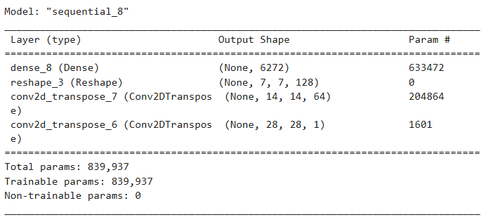
Generator Model
Step 6: Build the Discriminator Model
The Discriminator is responsible for distinguishing between real images from the dataset and fake images generated by the generator. It acts as a binary classifier that outputs the probability of whether an input image is real or fake.
- **Input: A 28 × 28 grayscale image is provided to the discriminator.
- **Convolutional Layers: These layers extract important visual features from the image, while dropout layers help reduce overfitting during training.
- **Flatten Layer: Converts the 3D feature maps into a 1D vector so it can be processed by fully connected layers.
- **Dense Layer: Produces the final classification output, determining whether the image is real or generated.
- **Output: A single probability value between 0 and 1, indicating the likelihood that the input image is real. R `
build_discriminator <- function() { model <- keras_model_sequential() %>% layer_conv_2d(filters = 64, kernel_size = c(5, 5), strides = c(2, 2), padding = 'same', activation = 'relu', input_shape = c(28, 28, 1)) %>% layer_dropout(rate = 0.3) %>% layer_conv_2d(filters = 128, kernel_size = c(5, 5), strides = c(2, 2), padding = 'same', activation = 'relu') %>% layer_dropout(rate = 0.3) %>% layer_flatten() %>% layer_dense(units = 1, activation = 'sigmoid')
return(model) }
discriminator <- build_discriminator()
summary(discriminator)
`
**Output:

Discriminator Model
Step 7: Compile the GAN Model
Here the Generator and Discriminator are combined to form the GAN model. The generator first produces synthetic images from random noise and these generated images are then evaluated by the discriminator. Both models are compiled using an optimizer and loss function for training.
R `
gan_input <- layer_input(shape = c(100))
x <- generator(gan_input)
gan_output <- discriminator(x)
gan_model <- keras_model(inputs = gan_input, outputs = gan_output) discriminator %>% compile( optimizer = optimizer_adam(), loss = 'binary_crossentropy', metrics = c('accuracy') )
gan_model %>% compile( optimizer = optimizer_adam(), loss = 'binary_crossentropy' )
`
Step 8: Discriminator Training Function
The discriminator needs to learn to distinguish real images from fake images generated by the generator. This function handles one training step for the discriminator:
- Generates fake images from random noise.
- Ensures the real and fake images have the same dimensions.
- Combines real and fake images and assigns labels (1 for real, 0 for fake).
- Trains the discriminator on this combined batch for one epoch. R `
batch_size <- 64 epochs <- 10 train_discriminator <- function(real_images, batch_size) {
noise <- matrix(rnorm(batch_size * 100), nrow = batch_size, ncol = 100) fake_images <- generator %>% predict(noise) if (length(dim(real_images)) == 3) { real_images <- array_reshape(real_images, c(batch_size, 28, 28, 1)) } print(dim(real_images)) print(dim(fake_images))
if (!identical(dim(real_images), dim(fake_images))) { stop("Dimension mismatch between real and fake images.") }
x_combined <- abind(real_images, fake_images, along = 1)
y_combined <- c(rep(1, batch_size), rep(0, batch_size))
d_loss <- discriminator %>% fit( x_combined, y_combined, epochs = 1, batch_size = batch_size, verbose = 0 )
return(d_loss) }
`
Step 9: Train the GAN
Here we handles the training loop for both the discriminator and generator. The generator tries to produce realistic images to fool the discriminator, while the discriminator learns to distinguish real from fake images.
- Generate a batch of real images from the dataset.
- Train the discriminator on the real images and fake images produced by the generator.
- Train the generator via the GAN model to fool the discriminator (using labels of 1).
- Repeat this process for the specified number of epochs, improving both networks iteratively. R `
train_gan <- function(batch_size) { noise <- matrix(rnorm(batch_size * 100), nrow = batch_size, ncol = 100) y_gan <- rep(1, batch_size) g_loss <- gan_model %>% fit(noise, y_gan, epochs = 1, batch_size = batch_size, verbose = 0) return(g_loss) }
for (epoch in 1:epochs) { cat(sprintf("Epoch %d\n", epoch)) real_batch <- generate_batch(x_train, batch_size) d_loss <- train_discriminator(real_batch, batch_size) cat(sprintf("Discriminator Loss: %.4f\n", d_loss$loss)) g_loss <- train_gan(batch_size) cat(sprintf("Generator Loss: %.4f\n", g_loss$loss)) if (epoch %% 10 == 0) { cat(sprintf("Epoch %d: Discriminator Loss: %.4f, Generator Loss: %.4f\n", epoch, d_loss$loss, g_loss$loss)) } }
`
**Output:
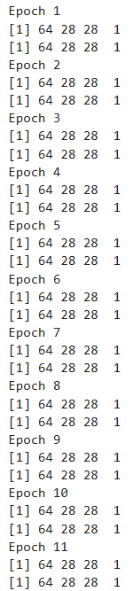
Traning GAN
Step 10: Generate and Visualize Images
After training the GAN, we can generate new synthetic images using the trained generator and visualize them. This helps to see how realistic the generated samples are compared to real data.
- Random noise vectors are fed into the generator to produce new images.
- The generator transforms the noise into 28×28 grayscale images. R `
generate_images <- function(num_images) { noise <- matrix(rnorm(num_images * 100), nrow = num_images, ncol = 100) generated_images <- generator %>% predict(noise) par(mfrow = c(1, num_images)) for (i in 1:num_images) { image(t(generated_images[i,,,1]), col = gray.colors(256), axes = FALSE, main = sprintf("Image %d", i)) } }
generate_images(5)
`
**Output:
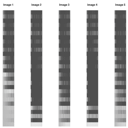
Output
Step 11: Track and Visualize Training Losses
After training a GAN, it’s important to monitor the losses of both the discriminator and generator to understand the training progress and detect issues like mode collapse or unstable training.
- During each epoch, the discriminator and generator losses are recorded.
- Using ggplot2, the losses are plotted over epochs to provide a clear picture of how both networks improve over time.
- Stable convergence of both losses indicates that the GAN is learning effectively. R `
library(ggplot2)
d_losses <- c() g_losses <- c() batch_size <- 64 epochs <- 10
for (epoch in 1:epochs) { real_batch <- generate_batch(x_train, batch_size) d_loss <- train_discriminator(real_batch, batch_size) d_losses <- c(d_losses, d_loss$loss) g_loss <- train_gan(batch_size) g_losses <- c(g_losses, g_loss$loss) cat(sprintf("Epoch %d - Discriminator Loss: %.4f, Generator Loss: %.4f\n", epoch, d_loss$loss, g_loss$loss)) }
plot_loss <- function(d_losses, g_losses) { if (length(d_losses) != length(g_losses)) stop("Loss vectors must have the same length") df <- data.frame(Epoch = 1:length(d_losses), Discriminator_Loss = d_losses, Generator_Loss = g_losses) ggplot(df, aes(x = Epoch)) + geom_line(aes(y = Discriminator_Loss, color = "Discriminator Loss")) + geom_line(aes(y = Generator_Loss, color = "Generator Loss")) + labs(title = "Training Losses", x = "Epoch", y = "Loss") + theme_minimal() }
plot_loss(d_losses, g_losses)
`
**Output:
Download full code from here
Applications
- **Image Generation: GANs can generate highly realistic images from random noise. They are widely used to create human faces, artwork and synthetic images that look similar to real-world data.
- **Image Super-Resolution: GANs can improve the quality of low-resolution images by generating higher-resolution versions. This is useful in areas such as medical imaging, satellite imagery and digital photography.
- **Data Augmentation: GANs can generate additional training data to increase the size of a dataset. This helps improve the performance of machine learning models, especially when real data is limited.
- **Video Generation: GANs can create realistic video sequences by generating frames that follow temporal patterns. This technology is used in video synthesis, animation and visual effects.
- **Image-to-Image Translation: GANs can convert one type of image into another, such as transforming sketches into realistic images or converting black-and-white images into colored ones.
Limitations
- **Training Instability: GANs are notoriously difficult to train. The adversarial process between the generator and discriminator can lead to oscillations or divergence if not carefully tuned.
- **High Computational Cost: Training GANs requires significant computational resources, especially for high-resolution images or complex datasets.
- **Sensitive to Hyperparameters: GAN performance heavily depends on the choice of learning rates, batch sizes and network architectures. Poor tuning can prevent convergence.
- **No Explicit Likelihood: Unlike some probabilistic models, GANs do not provide a direct way to compute likelihood, making evaluation and comparison more challenging.
- **Data Dependency: GANs require a large and representative dataset to generate high-quality outputs; limited data can lead to poor results.