Gradient Descent Algorithm in R (original) (raw)
Last Updated : 14 Apr, 2026
Gradient Descent is a optimization technique in machine learning that helps models learn by minimizing error. It works by iteratively adjusting parameters in the direction of the steepest decrease in the loss function. This process enables models like regression and neural networks to find the best weights for accurate predictions.
- Finds the direction where the error decreases the fastest.
- Updates the model parameters step by step to improve predictions.
- Helps models converge toward the best solution efficiently.
Gradient Descent
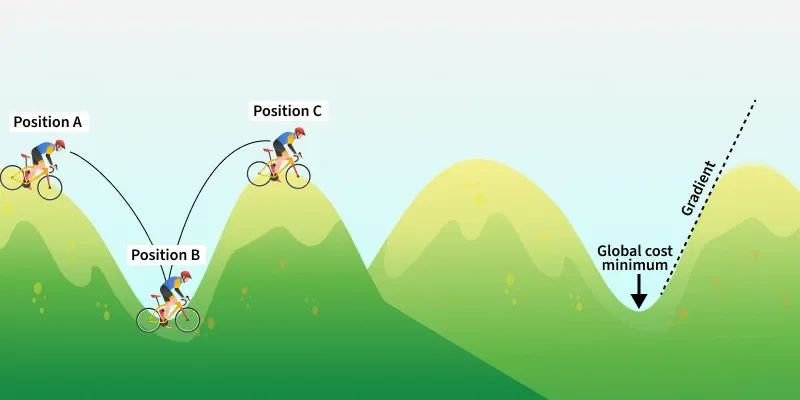
Gradient Descent is like descending a hill starting with random parameters, the slope (gradient) shows the steepest downward direction. By repeatedly stepping opposite the gradient, the algorithm gradually reaches the point of minimum error.
How Gradient Descent Works
Gradient Descent is an optimization algorithm that helps machine learning models find the best parameters to minimize error. The main goal is to reduce the difference between predicted and actual values by iteratively adjusting the model’s parameters in the direction of the steepest decrease in the cost function.
- Gradient Descent starts at an arbitrary point (random initial parameters) and evaluates the slope of the cost function.
- The slope or gradient, indicates the direction in which the function decreases fastest.
- By moving opposite to the gradient the algorithm gradually approaches the minimum of the cost function, also called the point of convergence.
- The process is similar to finding the line of best fit in linear regression, where the algorithm minimizes the error between predicted and actual outputs.
Role of Learning Rate
The learning rate (\alpha) controls the size of each step taken toward the minimum:
**1. Too small: The algorithm takes tiny steps, converges slowly and increases computational cost.
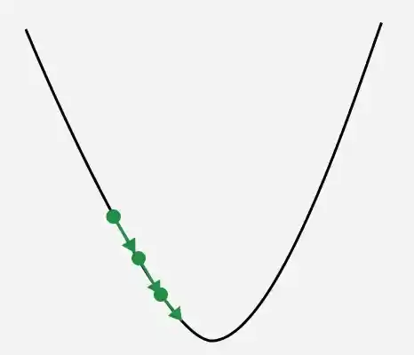
Learning rate with small steps
**2. Too large: The algorithm takes big steps, risks overshooting the minimum and may oscillate without converging due to a large learning rate. Exploding gradients, on the other hand, occur when gradients grow excessively large during backpropagation, leading to unstable updates.(exploding gradient problem).
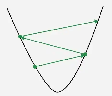
Learning rate with big steps
Choosing an appropriate learning rate ensures faster and stable convergence. Sometimes, Gradient Descent may face challenges like vanishing or exploding gradients. Techniques to mitigate these include:
- **Weight Regularization: Initialize weights carefully and use suitable activation functions like ReLU.
- **Gradient Clipping: Limit the gradient values to prevent extreme updates.
- **Batch Normalization: Normalize inputs at each layer to stabilize learning and prevent gradient problems.
Types of Gradient Descent
Gradient Descent can be categorized into different types based on how much training data is used to update the model parameters during each iteration.
Types of Gradient Descent
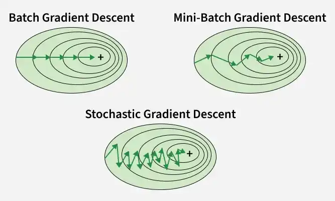
1.Batch Gradient Descent
Batch Gradient Descent updates the model parameters by computing the gradient of the loss function using the entire training dataset in each iteration.
- The algorithm computes the loss using all training examples in the dataset before updating the model parameters.
- The gradient is calculated from the entire dataset, which helps produce stable and accurate parameter updates.
- Batch Gradient Descent updates using all training samples, giving stable convergence but high computational cost for large datasets.
2. Stochastic Gradient Descent (SGD)
Stochastic Gradient Descent (SGD) updates the model parameters using one training example at a time, instead of computing the gradient over the entire dataset.
- The model parameters are updated immediately after processing each data point.
- This makes SGD faster for large datasets, but the updates can be noisy and may fluctuate around the minimum.
- SGD updates parameters frequently, allowing faster convergence and escape from local minima, but introduces noisy fluctuations in the loss.
3. Mini-batch Gradient Descent
Mini-Batch Gradient Descent is a hybrid approach that combines the advantages of Batch Gradient Descent and Stochastic Gradient Descent by updating model parameters using small subsets of the training data.
- The training dataset is divided into small groups called mini-batches.
- The gradient is computed using each mini-batch and the model parameters are updated after processing that batch.
- This method reduces the noise of SGD while remaining computationally efficient, making training faster and more stable.
Step By Step Implementation
Here we implement Gradient Descent algorithms for a linear regression problem in R Language.
Step 1: Generate a Synthetic Dataset
We create a synthetic dataset for linear regression. The dataset contains input values x and corresponding target values y with some random noise added.
R `
set.seed(42)
n <- 100 x <- runif(n, 0, 100) y <- 50 * x + 100 + rnorm(n, 0, 10)
`
Step 2: Initialize Model Parameters
Initialize the parameters of the linear regression model. These include the slope (m), intercept (b), learning rate and the number of iterations.
R `
m_init <- 0 b_init <- 0
alpha <- 0.00001 iterations <- 1000 batch_size <- 10
`
Step 3: Implement Batch Gradient Descent
In Batch Gradient Descent, the gradient is calculated using the entire dataset before updating the model parameters.
R `
batch_gd <- function(x, y, m, b, alpha, iterations){
n <- length(y) cost_history <- numeric(iterations)
for(i in 1:iterations){
y_pred <- m * x + b

gradient_m <- -(2/n) * sum(x * (y - y_pred))
gradient_b <- -(2/n) * sum(y - y_pred)

m <- m - alpha * gradient_m
b <- b - alpha * gradient_b

cost_history[i] <- mean((y - y_pred)^2)
}
return(list(m=m, b=b, cost_history=cost_history)) }
`
Step 4: Implement Stochastic Gradient Descent (SGD)
In SGD, the parameters are updated using one randomly selected data point at a time, which makes learning faster but introduces noise in the updates.
R `
sgd <- function(x, y, m, b, alpha, iterations){
n <- length(y) cost_history <- numeric(iterations)
for(i in 1:iterations){
idx <- sample(1:n,1)

x_i <- x[idx]
y_i <- y[idx]

y_pred <- m * x_i + b

gradient_m <- -2 * x_i * (y_i - y_pred)
gradient_b <- -2 * (y_i - y_pred)

m <- m - alpha * gradient_m
b <- b - alpha * gradient_b

y_full <- m * x + b
cost_history[i] <- mean((y - y_full)^2)
}
return(list(m=m, b=b, cost_history=cost_history)) }
`
Step 5: Implement Mini-Batch Gradient Descent
Mini-Batch Gradient Descent divides the dataset into small batches and updates the parameters after processing each batch.
R `
mini_batch_gd <- function(x, y, m, b, alpha, iterations, batch_size){
n <- length(y) cost_history <- numeric(iterations)
for(i in 1:iterations){
batch_index <- sample(1:n, batch_size)

x_batch <- x[batch_index]
y_batch <- y[batch_index]

y_pred <- m * x_batch + b

gradient_m <- -(2/batch_size) * sum(x_batch * (y_batch - y_pred))
gradient_b <- -(2/batch_size) * sum(y_batch - y_pred)

m <- m - alpha * gradient_m
b <- b - alpha * gradient_b

y_full <- m * x + b
cost_history[i] <- mean((y - y_full)^2)
}
return(list(m=m, b=b, cost_history=cost_history)) }
`
Step 6: Run the Gradient Descent Algorithms
Now we run the three gradient descent algorithms using the same dataset.
R `
batch_result <- batch_gd(x, y, m_init, b_init, alpha, iterations)
sgd_result <- sgd(x, y, m_init, b_init, alpha, iterations)
mini_result <- mini_batch_gd(x, y, m_init, b_init, alpha, iterations, batch_size)
`
Step 7: Visualize the Fitted Regression Lines
Here we visualize the regression lines learned by each gradient descent method.
R `
plot(x, y, main="Gradient Descent Regression Lines", xlab="x", ylab="y")
abline(batch_result$b, batch_result$m, col="red", lwd=2) abline(sgd_result$b, sgd_result$m, col="blue", lwd=2) abline(mini_result$b, mini_result$m, col="green", lwd=2)
legend("topleft", legend=c("Batch GD","SGD","Mini-Batch GD"), col=c("red","blue","green"), lwd=2)
`
**Output:
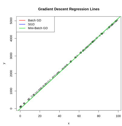
Regression Line
Step 8: Visualize Cost Convergence
Plot the cost function over iterations to observe how the algorithms converge during training.
R `
par(mfrow=c(3,1))
plot(batch_result$cost_history, type="l", col="red", lwd=2, xlab="Iterations", ylab="Cost", main="Batch Gradient Descent")
plot(sgd_result$cost_history, type="l", col="blue", lwd=2, xlab="Iterations", ylab="Cost", main="Stochastic Gradient Descent")
plot(mini_result$cost_history, type="l", col="green", lwd=2, xlab="Iterations", ylab="Cost", main="Mini-Batch Gradient Descent")
`
**Output:
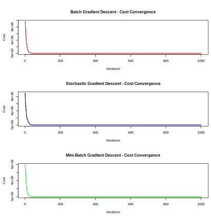
Cost Convergence
Step 9: Final Model Parameters
After training, we print the final learned parameters.
R `
cat("Batch GD -> m:", batch_result$m, " b:", batch_result$b, "\n") cat("SGD -> m:", sgd_result$m, " b:", sgd_result$b, "\n") cat("Mini Batch GD -> m:", mini_result$m, " b:", mini_result$b, "\n")
`
**Output:
Batch GD -> m: 51.42538 b: 1.215063
SGD -> m: 51.3787 b: 1.282832
Mini Batch GD -> m: 51.41466 b: 1.206799
Download full code from here
Applications of Gradient Descent
- **Neural Networks Training: Gradient Descent and its variants are used to update the weights and biases of neural networks during backpropagation to minimize the overall training loss.
- **Deep Learning Models: Modern deep learning architectures such as CNNs, RNNs and LSTMs rely on Gradient Descent-based optimizers to learn complex patterns from large datasets.
- **Recommendation Systems: Gradient Descent is used to optimize matrix factorization models in recommendation systems to predict user preferences and improve recommendations.
- **Natural Language Processing (NLP): Many NLP models use Gradient Descent to train embeddings, language models and text classification systems.
- **Computer Vision: Gradient Descent is applied to train image recognition models and optimize deep learning architectures used for object detection and image classification.
Limitations
- **Sensitive to Learning Rate: Choosing an appropriate learning rate is challenging. A very large learning rate can cause the algorithm to overshoot the minimum, while a very small learning rate can make the training process extremely slow.
- **Slow Convergence: Gradient Descent may require many iterations to converge, especially when dealing with large datasets or complex models.
- **Local Minima and Saddle Points: In non-convex optimization problems, the algorithm can get stuck in local minima or saddle points instead of reaching the global minimum.
- **High Computational Cost for Large Datasets: In Batch Gradient Descent, the gradient is computed using the entire dataset, which can be computationally expensive and slow when the dataset is very large.