Graph Convolutional Networks (GCNs): Architectural Insights and Applications (original) (raw)

Last Updated : 16 Apr, 2026

Graph Convolutional Networks (GCNs) have emerged as a powerful class of deep learning models designed to handle graph-structured data. Unlike traditional Convolutional Neural Networks (CNNs) that operate on grid-like data structures such as images, GCNs are tailored to work with non-Euclidean data, making them suitable for a wide range of applications including social networks, molecular structures and recommendation systems.

What-Are-Graph-Convolutional-Networks

Graph Convolutional Networks (GCNs)

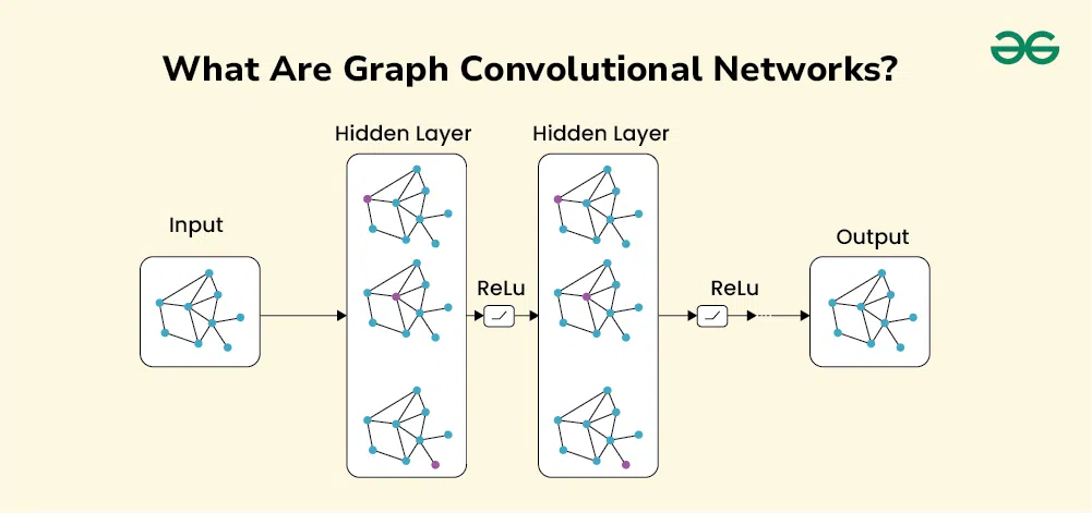
What Are Graph Convolutional Networks

Graph Convolutional Networks (GCNs) are a type of neural network designed to work directly with graphs. A graph consists of nodes (vertices) and edges (connections between nodes). In a GCN, each node represents an entity and the edges represent the relationships between these entities. The primary goal of GCNs is to learn node embeddings, which are vector representations of nodes that capture the graph's structural and feature information.

Architecture of GCNs

GCNs typically consist of multiple layers, each responsible for refining node embeddings by aggregating information from neighbors at increasing distances. The layers are:

Architecture-of-Graph-Convolutional-Networks-(GCNs)-

Architecture of GCNs

**1. Input Layer: The input layer initializes the node features, usually from raw data or pre-trained embeddings.

**2. Hidden Layers: Hidden layers perform the graph convolution operations, progressively aggregating and transforming node features.

**Graph Convolutional Layers: These layers perform the convolution operation on the graph. Each layer updates the feature representation of a node by aggregating the features of its neighbors.
**Activation Functions: Non-linear functions such as ReLU are applied to the output of each convolutional layer to introduce non-linearity into the model.
**Pooling Layers: These layers reduce the dimensionality of the graph by merging nodes, which helps in capturing hierarchical structures.

**3. Output Layer: The output layer produces the final node embeddings or predictions, depending on the task (e.g., node classification, link prediction).

**4. Fully Connected Layers: These layers are used at the end of the network to perform tasks such as classification or regression.

Types of Graph Convolutional Networks (GCNs)

GCNs can be broadly categorized into two types: Spectral-based and Spatial-based GCNs.

1. Spectral-based GCNs

Spectral-based GCNs are defined in the spectral domain using the graph Laplacian and Fourier transform. The convolution operation is performed by multiplying the graph signal with a filter in the spectral domain. This approach leverages the eigenvalues and eigenvectors of the graph Laplacian to perform convolution.

**Key Models:

**ChebNet: Uses Chebyshev polynomials to approximate the graph convolution operation, allowing for efficient computation on large graphs.
**GCN (Kipf & Welling): Simplifies the spectral convolution by using a first-order approximation, making it computationally efficient and scalable.

2. Spatial-based GCNs

Spatial-based GCNs perform convolution directly in the spatial domain by aggregating features from neighboring nodes. This approach is more intuitive and easier to implement compared to spectral-based methods.

**Key Models:

**GraphSAGE: Aggregates features from a fixed-size set of neighbors using mean, LSTM or pooling functions.
**GAT (Graph Attention Network): Introduces an attention mechanism to assign different weights to the neighbors of a node based on their importance.

How Graph Convolutional Networks (GCNs) Work

Step-by-step-working-of-GCNs-

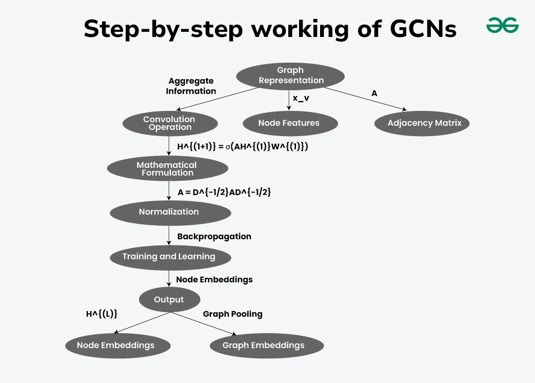
Graph Convolutional Networks (GCNs) Working

1. Graph Representation

**Nodes and Edges: Represent entities (nodes) and relationships (edges) between them using a graph G=(V,E) ,where V is the set of nodes and E is the set of edges.
**Node Features: Each node v∈V has associated features, x_v which could be initial attributes (e.g., text, images) or learned embeddings.

A graph G is represented by:

A set of nodes ?
A set of edges ?
An adjacency matrix ?, where ??? indicates the presence (and sometimes the weight) of an edge between node ? and node ?.

2. Convolution Operation on Graphs

In GCNs, the convolution operation is adapted to work on graphs. The key idea is to aggregate information from a node's neighbors to update its representation.

This process is analogous to the convolution operation in CNNs, which aggregates information from neighboring pixels.

3. Mathematical Formulation

The core operation in a GCN layer can be described by the following equation:

H^{(l+1)} = \sigma(\tilde{A} H^{(l)} W^{(l)})

where:

H^{(l)}is the matrix of node features at layer
\tilde{A} is the normalized adjacency matrix
W^{(l)} is the trainable weight matrix at layer
σ is an activation function, such as ReLU

4. Normalization

Normalization of the adjacency matrix \tilde{A} is crucial to ensure numerical stability and improve model performance. A common normalization technique is:

\tilde{A} = D^{-\frac{1}{2}} A D^{-\frac{1}{2}}

where ? is the degree matrix.

5. Training and Learning

**Backpropagation: GCNs are trained using gradient-based optimization methods (e.g., stochastic gradient descent) to minimize a loss function, typically tailored to the specific task (classification, regression, etc.).
**End-to-End Learning: The entire network, including convolutional layers and subsequent fully connected layers, is trained jointly to optimize performance on the task.

6. Output

**Node Embeddings: After several layers of graph convolution, the final node representations are used for downstream tasks like node classification or link prediction.
**Graph Embeddings: For graph-level tasks, additional aggregation or pooling over node embeddings can yield a single representation for the entire graph.

Training Graph Convolutional Networks (GCNs)

**Loss Functions: Training GCNs involves optimizing a loss function appropriate for the specific task. Common loss functions include cross-entropy loss for classification tasks and mean squared error for regression tasks
**Optimization: GCNs are trained using gradient-based optimization techniques such as stochastic gradient descent (SGD) or Adam. The gradients are computed through backpropagation, taking into account the graph structure.
**Regularization: To prevent overfitting, regularization techniques such as dropout and weight decay are applied. Dropout involves randomly setting a fraction of the node features to zero during training, while weight decay adds a penalty to the loss function based on the magnitude of the weights.

**Pseudocode for Graph Convolutional Networks (GCNs), is given below:

# Define the graph convolutional layer
def graph_convolutional_layer(A, X, W):
# A: Adjacency matrix of the graph
# X: Input feature matrix (N x D)
# W: Weight matrix (D x F)
# N: Number of nodes
# D: Number of input features per node
# F: Number of output features per node

# Calculate the degree matrix (D)
D = np.sum(A, axis=0)

# Calculate the normalized adjacency matrix (A_hat)
A_hat = A + np.eye(N)
D_hat = np.sqrt(D) + 1e-5
A_hat = A_hat / D_hat

# Calculate the output of the graph convolutional layer
output = np.dot(A_hat, X)
output = np.dot(output, W)

return output

# Define the GCN model
def GCN(A, X, W1, W2):
# A: Adjacency matrix of the graph
# X: Input feature matrix (N x D)
# W1: Weight matrix for the first layer (D x F1)
# W2: Weight matrix for the second layer (F1 x F2)
# N: Number of nodes
# D: Number of input features per node
# F1: Number of output features per node in the first layer
# F2: Number of output features per node in the second layer

# First graph convolutional layer
H1 = graph_convolutional_layer(A, X, W1)
H1 = np.maximum(H1, 0) # ReLU activation

# Second graph convolutional layer
H2 = graph_convolutional_layer(A, H1, W2)
H2 = np.maximum(H2, 0) # ReLU activation

return H2

Applications of Graph Convolutional Networks (GCNs)

**Social Networks: Friend recommendation (e.g., Facebook) using user connections
**Molecular Biology: Drug discovery by modeling molecules as graphs
**Knowledge Graphs: Entity classification (e.g., Google search understanding “Apple”)
**NLP: Semantic role labeling to understand sentence structure
**Computer Vision: Scene graph generation to detect objects and relationships

Variants and Extensions of Graph Convolutional Networks (GCNs)

**Graph Attention Networks (GATs): GATs extend GCNs by incorporating attention mechanisms, allowing the model to weigh the importance of different neighbors differently. This can lead to more accurate and expressive node embeddings.
**GraphSAGE: GraphSAGE (Graph Sample and Aggregation) improves the scalability of GCNs by sampling a fixed-size neighborhood for each node and aggregating information from these sampled neighbors. This approach is particularly useful for handling large graphs.
**ChebNet: ChebNet uses Chebyshev polynomials to approximate the graph convolution operation, reducing the computational complexity and enabling the use of higher-order neighborhoods.
**Graph Isomorphism Network (GIN): GINs are designed to be more expressive than traditional GCNs, ensuring that they can distinguish between different graph structures more effectively. This is achieved by incorporating a more powerful aggregation function.

Advantages and Disadvantages of GCNs

**Advantages of GCNs

**Efficient Handling of Irregular Data: Graph Convolutional Networks (GCNs) excel at processing irregular data structures, making them suitable for a wide range of applications beyond traditional grid data.
**Capturing Complex Relationships: By aggregating information from neighboring nodes, GCNs can capture complex relationships and dependencies, leading to more accurate and meaningful representations.
**Scalability: GCNs can be scaled to handle large graphs with millions of nodes and edges, making them applicable to real-world problems involving extensive data.

**Disadvantages of GCNs

**Scalability Issues: While GCNs can handle large graphs, scalability remains a challenge, especially for extremely large graphs. Techniques such as graph sampling and parallel processing are being explored to address this issue.
**Interpretability: Interpreting the learned node embeddings and understanding the decision-making process of GCNs can be difficult. Research is ongoing to develop methods that improve the interpretability of GCNs.
**Dynamic Graphs: Many real-world graphs are dynamic, with nodes and edges changing over time. Extending GCNs to effectively handle dynamic graphs is an active area of research.
**Combining GCNs with Other Models: Combining GCNs with other neural network architectures, such as recurrent neural networks (RNNs) or transformer models, can lead to more powerful hybrid models capable of tackling a broader range of tasks.