Image Segmentation Using UNet (original) (raw)

Last Updated : 20 Dec, 2025

U‑Net is a deep learning architecture designed specifically for image segmentation tasks. Its encoder‑decoder structure allows the model to capture both global context and fine‑grained details, making it highly effective for medical imaging, satellite imagery, and other pixel‑level classification problems.

• Uses skip connections for precise localization
• Works well with limited training data
• Delivers accurate segmentation results across diverse applications

Step By Step Implemenation

Here we will implement U-Net for semantic segmentation on a custom dataset containing RGB images and masks.

Step 1: Import Required Libraries

• NumPy is used for numerical computations.
• TensorFlow/Keras provides deep learning layers and models.
• Matplotlib and ImageIO help in visualization and image loading. Python `

import numpy as np import tensorflow as tf import os import imageio import matplotlib.pyplot as plt

from tensorflow.keras.layers import ( Input, Conv2D, MaxPooling2D, Dropout, Conv2DTranspose, concatenate ) from tensorflow.keras import Model from google.colab import drive

`

Step 2: Define Model Validation and Testing Utilities

• summary() extracts layer details for comparison.
• comparator() checks expected vs actual layers. Python `

from termcolor import colored

def comparator(learner, instructor): if len(learner) != len(instructor): raise AssertionError("Layer count mismatch") for a, b in zip(learner, instructor): if tuple(a) != tuple(b): print(colored("Test failed", attrs=['bold'])) raise AssertionError("Error in test") print(colored("All tests passed!", "green"))

def summary(model): result = [] for layer in model.layers: output_shape = getattr(layer.output, 'shape', None) params = layer.count_params() if hasattr(layer, 'count_params') else 0 result.append([layer.class.name, output_shape, params]) return result

`

Step 3: Mount Google Drive and Load Dataset Paths

• Google Drive is mounted for accessing image data.
• Image and mask directories are defined.
• File paths are filtered and sorted.

You can download Image Segmentation Dataset from Kaggle

Python `

drive.mount('/content/drive')

image_path = "/content/drive/MyDrive/CameraRGB" mask_path = "/content/drive/MyDrive/CameraMask"

image_list = sorted([os.path.join(image_path, f) for f in os.listdir(image_path) if f.endswith('.png')]) mask_list = sorted([os.path.join(mask_path, f) for f in os.listdir(mask_path) if f.endswith('.png')])

`

Step 4: Visualize Sample Image and Mask

• Displays the image and its mask side by side using subplots.
• Supports both 2D and 3D masks, shown in grayscale with axes hidden. Python `

N = 2 img = imageio.imread(image_list[N]) mask = imageio.imread(mask_list[N])

fig, ax = plt.subplots(1, 2, figsize=(12, 6)) ax[0].imshow(img) ax[0].set_title("Image") ax[0].axis("off")

ax[1].imshow(mask[:, :, 0] if mask.ndim == 3 else mask, cmap="gray") ax[1].set_title("Mask") ax[1].axis("off") plt.show()

`

**Output:

Step 5: Create TensorFlow Dataset

• Converts image and mask file paths into TensorFlow constant tensors.
• Pairs each image path with its corresponding mask path.
• Creates a TensorFlow dataset using from_tensor_slices for efficient data loading. Python `

image_filenames = tf.constant(image_list) mask_filenames = tf.constant(mask_list)

dataset = tf.data.Dataset.from_tensor_slices((image_filenames, mask_filenames))

`

Step 6: Dataset Preprocessing Pipeline

• process_path( ) reads image and mask files from disk, decodes them and converts them into tensors
• preprocess( ) resizes image and mask, normalizes the image and prepares them for model input Python `

def process_path(image_path, mask_path): img = tf.io.read_file(image_path) img = tf.image.decode_png(img, channels=3) img = tf.image.convert_image_dtype(img, tf.float32)

mask = tf.io.read_file(mask_path)
mask = tf.image.decode_png(mask, channels=3)
mask = tf.math.reduce_max(mask, axis=-1, keepdims=True)
return img, mask

def preprocess(image, mask): input_image = tf.image.resize(image, (96, 128), method='nearest') input_mask = tf.image.resize(mask, (96, 128), method='nearest')

input_image = input_image / 255.

return input_image, input_mask

image_ds = dataset.map(process_path) processed_image_ds = image_ds.map(preprocess)

`

Step 7: U-Net Building Blocks (Encoder and Decoder)

• conv_block( ) extracts features using two convolution layers and returns a pooled output with a skip connection.
• upsampling_block( ) upsamples feature maps using transposed convolution and merges them with encoder features.
• Applies two convolutions after concatenation to refine spatial details in the decoder path. Python `

def conv_block(inputs, n_filters, dropout_prob=0, max_pooling=True): conv = Conv2D(n_filters, 3, activation='relu', padding='same', kernel_initializer='he_normal')(inputs) conv = Conv2D(n_filters, 3, activation='relu', padding='same', kernel_initializer='he_normal')(conv)

if dropout_prob > 0:
    conv = Dropout(dropout_prob)(conv)

next_layer = MaxPooling2D((2, 2))(conv) if max_pooling else conv
skip_connection = conv
return next_layer, skip_connection

def upsampling_block(expansive_input, contractive_input, n_filters): up = Conv2DTranspose(n_filters, 3, strides=2, padding='same')(expansive_input) merge = concatenate([up, contractive_input], axis=3)

conv = Conv2D(n_filters, 3, activation='relu', padding='same',
              kernel_initializer='he_normal')(merge)
conv = Conv2D(n_filters, 3, activation='relu', padding='same',
              kernel_initializer='he_normal')(conv)
return conv

`

Step 8: Build the U-Net Model

• Defines the U-Net architecture with encoder, bottleneck and decoder using skip connections.
• Initializes the model with a 96×128 RGB input and multi-class output.
• Compiles the model using Adam optimizer and Sparse Categorical Crossentropy loss.
• Displays the model summary showing layers, parameters and output shapes. Python `

def unet_model(input_size=(96,128,3), n_filters=32, n_classes=23): inputs = Input(input_size)

c1 = conv_block(inputs, n_filters)
c2 = conv_block(c1[0], n_filters*2)
c3 = conv_block(c2[0], n_filters*4)
c4 = conv_block(c3[0], n_filters*8, dropout_prob=0.3)
c5 = conv_block(c4[0], n_filters*16, dropout_prob=0.3, max_pooling=False)

u6 = upsampling_block(c5[0], c4[1], n_filters*8)
u7 = upsampling_block(u6, c3[1], n_filters*4)
u8 = upsampling_block(u7, c2[1], n_filters*2)
u9 = upsampling_block(u8, c1[1], n_filters)

outputs = Conv2D(n_classes, 1, activation='softmax')(u9)
return Model(inputs, outputs)

unet = unet_model() unet.compile( optimizer='adam', loss=tf.keras.losses.SparseCategoricalCrossentropy(from_logits=True), metrics=['accuracy'] ) unet.summary()

`

**Output:

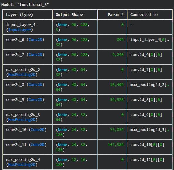
Unet Model

Step 9: Train U-Net Model

• Hyperparameters like epochs, batch size, buffer size and validation splits are set for training.
• Dataset is cached, shuffled and batched for efficient training.
• The U-Net model is trained on the prepared dataset using fit() for the specified number of epochs. Python `

EPOCHS = 40 VAL_SUBSPLITS = 5 BUFFER_SIZE = 500 BATCH_SIZE = 32 processed_image_ds.batch(BATCH_SIZE) train_dataset = processed_image_ds.cache().shuffle(BUFFER_SIZE).batch(BATCH_SIZE) print(processed_image_ds.element_spec) model_history = unet.fit(train_dataset, epochs=EPOCHS)

`

**Output:

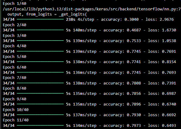
Unet Traning

Step 10: Training Accuracy Visualization

Plots how the model’s accuracy changes over epochs during training.

Python `

plt.plot(model_history.history["accuracy"])

`

**Output:

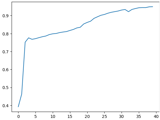
Training Accuracy

Step 11: Visualizing U-Net Predictions

• show_predictions displays input images, ground truth masks and predicted masks side by side.
• Uses create_mask to convert model output probabilities into single-channel masks for visualization.
• Helps qualitatively assess model performance on training or sample data. Python `

def create_mask(pred_mask): pred_mask = tf.argmax(pred_mask, axis=-1) pred_mask = pred_mask[..., tf.newaxis] return pred_mask[0] def show_predictions(dataset=None, num=1): if dataset: for image, mask in dataset.take(num): pred_mask = unet.predict(image) display([image[0], mask[0], create_mask(pred_mask)]) else: display([sample_image, sample_mask, create_mask(unet.predict(sample_image[tf.newaxis, ...]))])

show_predictions(train_dataset, 6)

`

**Output:

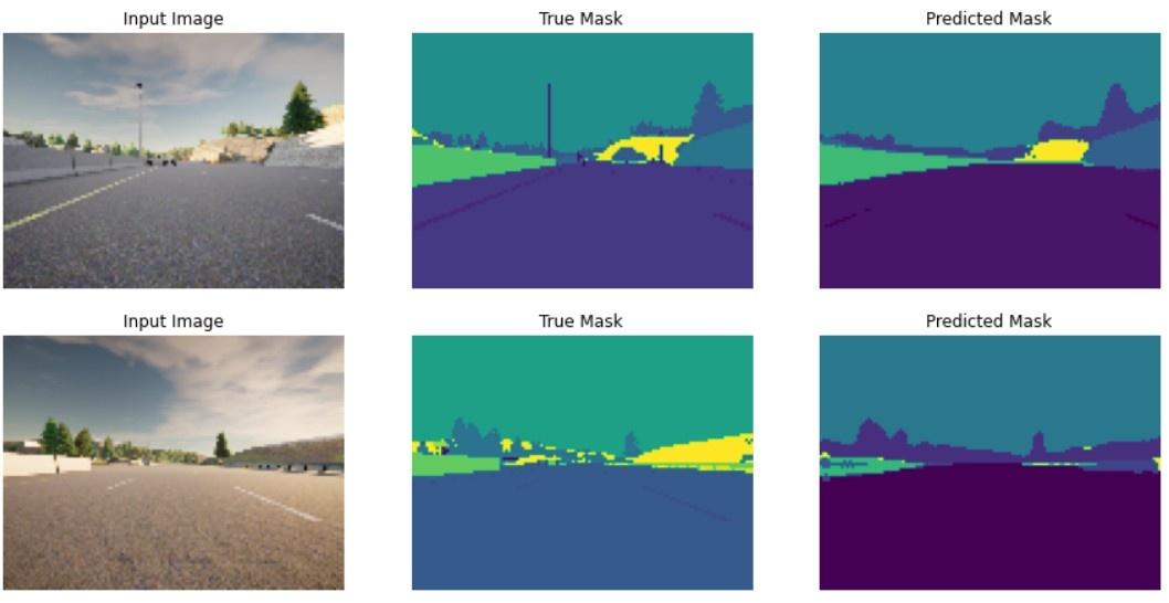
Output

We an see our model is working fine.

You can download full code from here