Long ShortTerm Memory (LSTM) using R (original) (raw)
Long Short-Term Memory (LSTM) using R
Last Updated : 14 Apr, 2026
Long Short-Term Memory (LSTM) networks are neural networks designed for sequential data like time series, text or speech. Unlike traditional RNNs, which struggle with vanishing or exploding gradients, LSTMs use gates to store, update and retrieve information, enabling them to capture long-term dependencies effectively.
- Stores information across time steps to capture long-term dependencies.
- Uses input, forget and output gates to control information flow.
- Handles long sequences effectively without vanishing gradient issues.
Problem with Long-Term Dependencies in RNN
Recurrent Neural Networks (RNNs) are designed to process sequential data by maintaining a memory of previous time steps. However they often struggle to capture information from distant past steps, which is important for accurate predictions.
- **Vanishing Gradient: When training over long sequences the gradients that help the network learn can shrink as they pass through many steps. This makes it difficult for the model to learn long-term patterns since earlier information becomes almost irrelevant.
- **Exploding Gradient: Sometimes the gradients grow too large, causing instability during training. This results in erratic updates, making it hard for the model to learn properly.
- **Impact on RNNs: Both vanishing and exploding gradients prevent standard RNNs from effectively remembering and using information from earlier time steps, limiting their ability to capture long-term dependencies.
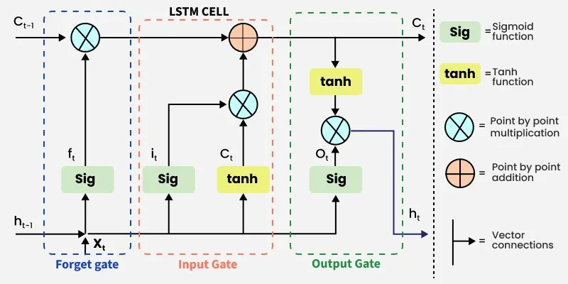
LSTM Architecture
Long Short-Term Memory (LSTM) networks have a specialized architecture designed to capture long-term dependencies in sequential data. The core of an LSTM is the memory cell, which acts as the network’s long-term memory. The memory cell is controlled by three gates that regulate the flow of information:
LSTM Architecture
- **Input Gate: Decides which new information from the current input and previous hidden state should be added to the memory cell.
- **Forget Gate: Determines which information in the memory cell should be discarded, allowing the network to remove irrelevant or outdated data.
- **Output Gate: Controls which part of the memory cell is sent to the hidden state as output for the current time step.
The LSTM also maintains a hidden state acts as short-term memory and is updated at each time step using the current input, previous hidden state and memory cell. This allows LSTMs to selectively retain, update or discard information, capturing both short-term and long-term patterns.
Working of LSTM
LSTM networks have a chain-like architecture consisting of memory blocks called cells and multiple neural networks. The memory cell retains information, while gates regulate what information is added, removed or output at each time step. There are three main gates in an LSTM:
**1. Forget Gate
The forget gate determines which information from the previous cell state should be discarded. This prevents irrelevant or outdated information from accumulating in the memory.
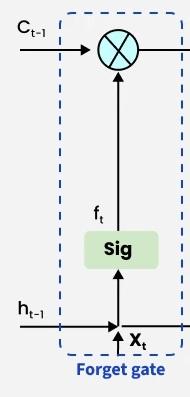
Forget gate
- Inputs are the Previous hidden state h_{t-1} and current input x_{t}.
- The inputs are multiplied by a weight matrix, bias is added and the result is passed through a sigmoid activation \sigma, producing values between 0 and 1.
- A value near 0 means the corresponding information is discarded, while a value near 1 means it is retained.
The forget gate is computed as:
f_t = \sigma\left(W_f \cdot [h_{t-1}, x_t] + b_f\right)
where
- W_{f} is the weight matrix for the forget gate.
- [h_{t-1},x_{t}] is the concatenation of previous hidden state and current input.
- b_{f} is the bias term.
- \sigma is the sigmoid function, giving outputs in the range [0,1].
**2. Input Gate
The input gate decides what new information should be added to the cell state. It also takes x_{t} and h_{t-1}. as inputs.
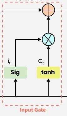
Input gate
The process involves two steps:
**Regulation: A sigmoid function filters which parts of the input should influence the cell state.
i_t = \sigma\left(W_i \cdot [h_{t-1}, x_t] + b_i\right)
**Candidate Values: A tanh function generates a vector of new candidate values that could be added to the cell state.
\hat{C_{t}} = \tanh\left(W_c \cdot [h_{t-1}, x_t] + b_c\right)
The previous cell state C_{t-1} is first filtered by the forget gate f_{t} (removing unneeded information), then the candidate values are scaled by i_{t} and added:
C_t = f_t \odot C_{t-1} + i_t \odot \hat{C_{t}}
Here \odot represents element-wise multiplication. This ensures only relevant new information is added to the cell state.
This ensures the memory cell only updates with relevant new information while retaining important old information.
**3. Output gate
The output gate is responsible for deciding what part of the current cell state should be sent as the hidden state (output) for this time step.
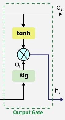
Output gate
First, the gate uses a sigmoid function to determine which information from the current cell state will be output. This is done using the previous hidden state h_{t-1} and the current input x_{t}.
o_t = \sigma\left(W_o \cdot [h_{t-1}, x_t] + b_o\right)
Next, the current cell state C_{t} is passed through a tanh activation to scale its values between −1 and +1. Finally, this transformed cell state is multiplied element-wise with o_{t} to produce the hidden state h_{t}:
h_t = o_t \odot \tanh(C_t)
where
- o_{t}is the output gate activation.
- C_{t} is the current cell state.
This hidden state h_{t} is then passed to the next time step and can also be used for generating the output of the network.
Step By Step Implementation
Here we implement LSTM networks in R using the Keras library, which provides a high-level interface for building and training neural networks.
Step 1: Install and Load Required Libraries
Install the required packages and load the Keras and TensorFlow libraries. These libraries are used to build and train deep learning models in R.
R `
install.packages("keras") install.packages("tensorflow")
library(keras) library(tensorflow)
install_tensorflow()
`
Step 2: Prepare the Training Dataset
Create a sample dataset for training the LSTM model. The input data is generated as a 3D array (samples, timesteps, features) and the labels are converted into categorical format using one-hot encoding.
R `
X_train <- array(runif(1000), dim = c(100, 10, 10)) labels <- sample(0:9, 100, replace = TRUE) y_train <- to_categorical(labels, num_classes = 10)
`
Step 3: Define the LSTM Model
Here we define the neural network architecture using the Sequential API. The model includes an LSTM layer followed by a Dense output layer with softmax activation.
R `
model <- keras_model_sequential() %>% layer_lstm( units = 50, input_shape = c(10, 10) ) %>% layer_dense( units = 10, activation = "softmax" )
`
Step 4: Compile and Inspect the Model
Before training, compile the model by specifying the loss function, optimizer and evaluation metric and then display the model architecture.
R `
model %>% compile( loss = "categorical_crossentropy", optimizer = optimizer_adam(), metrics = c("accuracy") )
summary(model)
`
**Output:
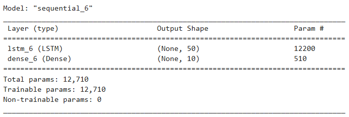
Model Architecture
Step 5: Train the LSTM Model
Train the model using the training dataset by specifying the number of epochs, batch size and validation split.
R `
history <- model %>% fit( X_train, y_train, epochs = 10, batch_size = 32, validation_split = 0.2 )
`
Step 6: Evaluate the Model
After training the model, we evaluate its performance on the dataset to measure the loss and accuracy of the trained LSTM model
R `
score <- model %>% evaluate(X_train, y_train)
print(score)
cat("Test loss:", score["loss"], "\n") cat("Test accuracy:", score["accuracy"], "\n")
`
**Output:
loss accuracy
2.227077 0.160000
Test loss: 2.227077
Test accuracy: 0.16
Step 7: Generate Predictions
We use the trained model to generate predictions for the input data. The output shows the predicted probabilities for each class.
R `
predictions <- model %>% predict(X_train) print(predictions[1,])
`
**Output:
[1] 0.09753080 0.14767092 0.12659180 0.04785443 0.06404027 0.07024606
[7] 0.12305354 0.10367487 0.13839653 0.08094072
Download full code from here.
Applications
- **Language Translation: Sequence-to-sequence LSTM models are used in machine translation systems like Google Translate, learning to convert text from one language to another while preserving context and meaning.
- **Sentiment Analysis: LSTMs can understand the context and relationships between words to classify text based on sentiment, useful for analyzing customer feedback or social media content.
- **Text Summarization: By focusing on the most important information in a text, LSTMs can generate concise summaries for documents, articles or reports.
- **Language Modeling: LSTMs learn dependencies between words to generate coherent and grammatically correct sentences, supporting tasks like predictive text and autocomplete.
- **Time Series Forecasting: LSTMs predict future events in sequential data, such as stock prices, weather or energy consumption.
- **Anomaly Detection: They detect unusual patterns in data, which is useful for fraud detection, network intrusion detection or system monitoring.
Limitations
- **Computationally Expensive: LSTMs have complex architectures with multiple gates and weight matrices, which makes training slower and requires more computational resources compared to simpler models.
- **Difficult to Tune: LSTMs have many hyperparameters, such as number of layers, hidden units, learning rate and dropout, which makes model tuning challenging and time-consuming.
- **Memory-Intensive: Large sequence lengths or high-dimensional input data can result in high memory usage during training.
- **Limited Parallelization: LSTM computations are inherently sequential, which makes them harder to parallelize, slowing down training on long sequences.
- **Overfitting Risk: LSTMs can overfit on small datasets because of their high capacity and large number of parameters.