Long Short Term Memory (LSTM) Networks using PyTorch (original) (raw)
Last Updated : 9 Oct, 2025
Long Short-Term Memory (LSTM) networks are a special type of Recurrent Neural Network (RNN) designed to address the vanishing gradient problem, which makes it difficult for traditional RNNs to learn long-term dependencies in sequential data.

LSTM Networks using PyTorch
LSTMs use memory cells controlled by three gates:
- **Input Gate: decides what new information should be stored.
- **Forget Gate: decides what information should be discarded.
- **Output Gate: decides what information to output at each step.
This structure allows LSTMs to remember useful information for long periods while ignoring irrelevant details. In this article, we will learn how to implement an LSTM in PyTorch for sequence prediction on synthetic sine wave data.
Long Short-Term Memory (LSTM) Networks using PyTorch
LSTMs are widely used for sequence modeling tasks because of their ability to capture long-term dependencies. PyTorch provides a clean and flexible API to build and train LSTM models. In PyTorch, the nn.LSTM module handles the recurrence logic, while the rest of the architecture (such as fully connected layers, dropout, etc.) can be customized as needed.
Key Components
**1. Input Size: Number of features in the input sequence at each time step.
**2. Hidden Size: Number of features in the hidden state.
**3. Number of Layers: Stacking multiple LSTM layers deepens the model.
**4. Batch First: If set to True, input/output tensors are provided as (batch, seq_len, features) instead of (seq_len, batch, features).
**5. Outputs:
- **Output Sequence: Hidden states at each time step.
- **Hidden State: Final hidden state for all layers.
- **Cell State: Final memory cell state for all layers.
Implementation
Let's implement LSTM network using PyTorch,
Step 1: Import Libraries and Prepare Data
We first import the necessary libraries such as torch, numpy and matplotlib and create a sine wave dataset. The data is split into input sequences of length 10, where the model predicts the next value.
- **np.linspace(): generates evenly spaced points.
- **np.sin(): creates sine values.
- **create_sequences(): prepares input-output pairs.
- **torch.tensor(): converts NumPy arrays into PyTorch tensors. Python `
import torch import torch.nn as nn import numpy as np import matplotlib.pyplot as plt
np.random.seed(0) torch.manual_seed(0)
t = np.linspace(0, 100, 1000) data = np.sin(t)
def create_sequences(data, seq_length): xs, ys = [], [] for i in range(len(data) - seq_length): x = data[i:(i + seq_length)] y = data[i + seq_length] xs.append(x) ys.append(y) return np.array(xs), np.array(ys)\
seq_length = 10 X, y = create_sequences(data, seq_length)
trainX = torch.tensor(X[:, :, None], dtype=torch.float32) trainY = torch.tensor(y[:, None], dtype=torch.float32)
`
Step 2: Define the LSTM Model
We define an LSTM model using PyTorch’s nn.Module.
- **nn.LSTM: processes sequential data.
- **nn.Linear: maps hidden state outputs to predictions.
- **forward(): runs the data through LSTM + Fully Connected layer. Python `
class LSTMModel(nn.Module): def init(self, input_dim, hidden_dim, layer_dim, output_dim): super(LSTMModel, self).init() self.hidden_dim = hidden_dim self.layer_dim = layer_dim self.lstm = nn.LSTM(input_dim, hidden_dim, layer_dim, batch_first=True) self.fc = nn.Linear(hidden_dim, output_dim)
def forward(self, x, h0=None, c0=None):
    if h0 is None or c0 is None:
        h0 = torch.zeros(self.layer_dim, x.size(
            0), self.hidden_dim).to(x.device)
        c0 = torch.zeros(self.layer_dim, x.size(
            0), self.hidden_dim).to(x.device)

    out, (hn, cn) = self.lstm(x, (h0, c0))
    out = self.fc(out[:, -1, :])  # Take last time step
    return out, hn, cn
`
Step 3: Initialize Model, Loss Function, and Optimizer
- **Model: 1 input, 100 hidden units, 1 LSTM layer, 1 output.
- **Loss Function: Mean Squared Error (MSE) for regression.
- **Optimizer: Adam optimizer for efficient training. Python `
model = LSTMModel(input_dim=1, hidden_dim=100, layer_dim=1, output_dim=1) criterion = nn.MSELoss() optimizer = torch.optim.Adam(model.parameters(), lr=0.01)
`
Step 4: Train the LSTM Model
We train the model for 100 epochs.
- **Forward pass: model makes predictions.
- **Loss calculation: compare predicted vs. actual values.
- **Backpropagation: update weights.
- **Detach hidden states: prevent gradient buildup. Python `
num_epochs = 100 h0, c0 = None, None
for epoch in range(num_epochs): model.train() optimizer.zero_grad()
outputs, h0, c0 = model(trainX, h0, c0)

loss = criterion(outputs, trainY)
loss.backward()
optimizer.step()

h0, c0 = h0.detach(), c0.detach()

if (epoch + 1) % 10 == 0:
    print(f'Epoch [{epoch+1}/{num_epochs}], Loss: {loss.item():.4f}')
`
**Output:
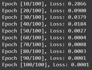
Training
Step 5: Evaluate and Plot Predictions
We evaluate model using model.eval() and get the predicted outputs.
Python `
model.eval() predicted, _, _ = model(trainX, h0, c0)
original = data[seq_length:] time_steps = np.arange(seq_length, len(data))
predicted[::30] += 0.2 predicted[::70] -= 0.2
plt.figure(figsize=(12, 6)) plt.plot(time_steps, original, label='Original Data') plt.plot(time_steps, predicted.detach().numpy(), label='Predicted Data', linestyle='--') plt.title('LSTM Model Predictions vs. Original Data') plt.xlabel('Time Step') plt.ylabel('Value') plt.legend() plt.show()
`
**Output:
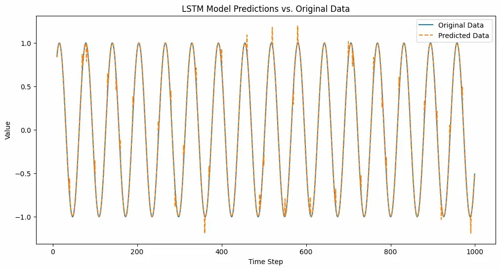
Plot
Applications
- **Natural Language Processing (NLP): Machine translation, text generation, sentiment analysis, and speech-to-text.
- **Time-Series Forecasting: Stock price prediction, weather forecasting, energy demand forecasting.
- **Healthcare: Patient monitoring (heart rate, ECG), disease progression modeling, medical event prediction.
- **Finance: Credit risk analysis, fraud detection, algorithmic trading.
- **Speech & Audio Processing: Speech recognition, voice assistants, music generation.
- **Anomaly Detection: Detecting unusual patterns in IoT sensors, cybersecurity logs, or industrial equipment.
Advantages
- **Easy Debugging: Dynamic computation graphs allow native Python debugging.
- **Flexible Architecture: Works well with varying input lengths.
- **Balanced API: Provides both high- and low-level control.
- **Strong Backing: Maintained by Meta with frequent updates.
- **Active Community: Large ecosystem of tutorials and examples.
Limitations
- **Less Mature than TensorFlow: Fewer enterprise-level tools.
- **Fewer Advanced Resources: Limited high-level tutorials for LSTMs.
- **Manual Optimization: Requires tuning for best performance.
- **Version Gaps: API changes may affect older code.