Lung Cancer Detection using Convolutional Neural Network (CNN) (original) (raw)

Last Updated : 10 Apr, 2026

Computer Vision is one of the applications of deep neural networks and one such use case is in predicting the presence of cancerous cells. In this article, we will learn how to build a classifier using Convolution Neural Network which can classify normal lung tissues from cancerous tissues.

The following process will be followed to build this classifier:

importing_libraries_dataset

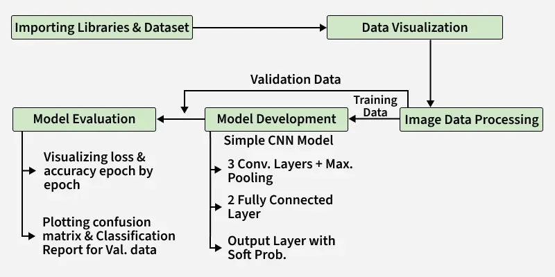
Process

Implementation

Step 1: Importing Libraries

We use libraries for data handling, visualization and deep learning model development.

Pandas, NumPy, Matplotlib and Scikit-learn for data handling and analysis.
OpenCV for image processing.
TensorFlow to build and train machine learning models, including CNNs. Python `

import os import random import cv2 import numpy as np import pandas as pd import matplotlib.pyplot as plt from PIL import Image

from sklearn.model_selection import train_test_split from sklearn import metrics

import tensorflow as tf from tensorflow import keras from keras import layers

import warnings warnings.filterwarnings('ignore')

Step 2: Importing Dataset

The dataset used is a custom subset (~2400images) containing three lung cancer categories

Normal (lung_n)
Adenocarcinoma (lung_aca)
Squamous cell carcinoma (lung_scc) Python `

data_path = 'lung_subset_small_folder.zip' with ZipFile(data_path, 'r') as zip: zip.extractall() print('The data set has been extracted.')

**Output:

The data set has been extracted.

Step 3: Visualizing the Data

We visualize random images from each category to understand the dataset.

Python `

path = 'lung_subset_small'

classes = ['lung_n', 'lung_aca', 'lung_scc']

for cat in classes: image_dir = f'{path}/{cat}' images = os.listdir(image_dir)

fig, ax = plt.subplots(1, 3, figsize=(15, 5))
fig.suptitle(f'Images for {cat} category . . . .', fontsize=20)

for i in range(3):
    k = np.random.randint(0, len(images))
    img = np.array(Image.open(f'{path}/{cat}/{images[k]}'))
    ax[i].imshow(img)
    ax[i].axis('off')
plt.show()

**Output:

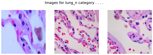
Images for lung_n category

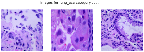
Images for lung_aca category

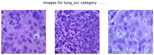
Images for lung_scc category

Step 4: Preparing the Dataset

Instead of loading all images into memory, we use ImageDataGenerator to load images batch-by-batch.

Rescales pixel values
Splits data into training (80%) and validation (20%)
Prevents memory overflow Python `

IMG_SIZE = 128
BATCH_SIZE = 16
EPOCHS = 10

datagen = ImageDataGenerator( rescale=1./255, validation_split=0.2 )

train_data = datagen.flow_from_directory( path, target_size=(IMG_SIZE, IMG_SIZE), batch_size=BATCH_SIZE, class_mode='categorical', subset='training' )

val_data = datagen.flow_from_directory( path, target_size=(IMG_SIZE, IMG_SIZE), batch_size=BATCH_SIZE, class_mode='categorical', subset='validation' )

**Output:

output

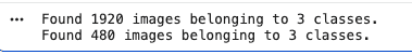
Output

Step 5: Model Development

Now we start building the CNN. Here, we use TensorFlow and Keras to define the architecture of our CNN model.

**Sequential(): Builds a linear stack of layers.
**Conv2D(): Applies convolution with specified filters, kernel size, ReLU activation and padding.
**MaxPooling2D(): Downsamples feature maps by taking max values over pool size.
**Flatten(): Converts 2D feature maps into 1D vector.
**Dense(): Fully connected layer with given units and activation.
**BatchNormalization(): Normalizes activations to speed up training.
**Dropout(): Randomly drops neurons to reduce overfitting.
**model.summary(): Displays model architecture details. Python `

model = keras.models.Sequential([ layers.Conv2D(32, (5, 5), activation='relu', padding='same', input_shape=(IMG_SIZE, IMG_SIZE, 3)), layers.MaxPooling2D(2, 2),

layers.Conv2D(64, (3, 3), activation='relu', padding='same'),
layers.MaxPooling2D(2, 2),

layers.Conv2D(128, (3, 3), activation='relu', padding='same'),
layers.MaxPooling2D(2, 2),

layers.Flatten(),
layers.Dense(256, activation='relu'),
layers.BatchNormalization(),
layers.Dense(128, activation='relu'),
layers.Dropout(0.3),
layers.BatchNormalization(),
layers.Dense(3, activation='softmax')

])

model.summary()

**Output:

output2

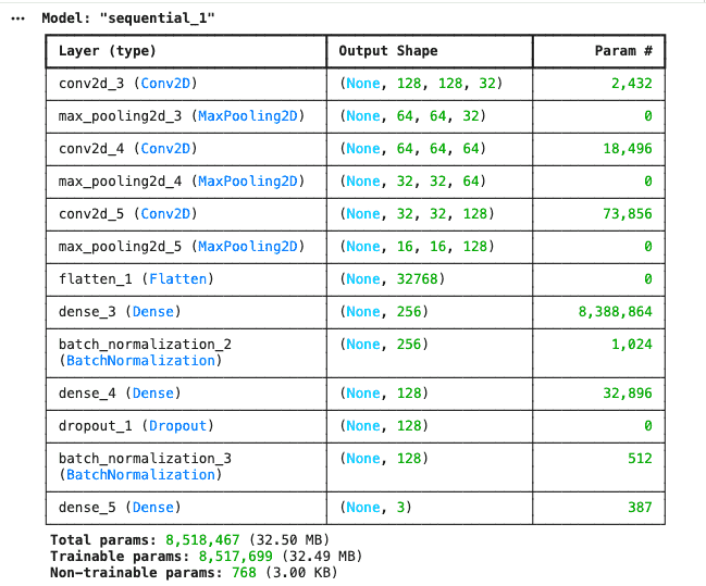
Output

Step **6: Model Compilation

After defining the model architecture we will compile the model with an optimizer, loss function and evaluation metric then train it using the training data.

We use the Adam optimizer which adjusts the learning rate during training to speed up convergence.
Categorical cross entropy loss is appropriate as loss function for multi-class classification problems as it measures the difference between the predicted and actual probability distributions.
**EarlyStopping: Stops training if validation accuracy doesn’t improve for a set number of epochs (patience).
**ReduceLROnPlateau: Reduces learning rate when validation loss plateaus, controlled by patience and factor.
**Custom myCallback class: Stops training early when validation accuracy exceeds 90%.
**self.model.stop_training = True: Signals to stop training inside the callback. Python `

from keras.callbacks import EarlyStopping, ReduceLROnPlateau

class myCallback(tf.keras.callbacks.Callback): def on_epoch_end(self, epoch, logs=None): if logs.get('val_accuracy') > 0.90: print("Stopping early") self.model.stop_training = True

es = EarlyStopping(patience=3, monitor='val_accuracy', restore_best_weights=True)

lr = ReduceLROnPlateau(monitor='val_loss', patience=2, factor=0.5)

model.compile( optimizer='adam', loss='categorical_crossentropy', metrics=['accuracy'] )

Step 7: Model Training

The model is trained using generator-based data.

Python `

history = model.fit( train_data, validation_data=val_data, epochs=EPOCHS, callbacks=[es, lr, myCallback()] )

**Output:

output3

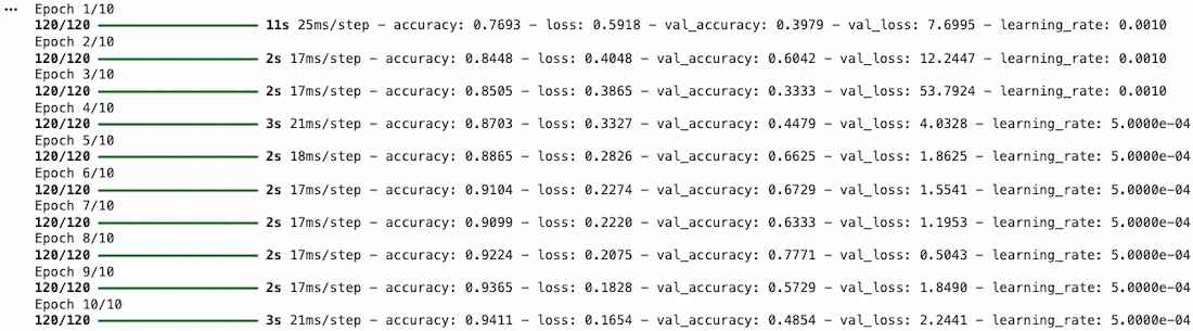
Training

Step 8: Visualizing

Let's visualize the training and validation accuracy with each epoch.

pd.DataFrame(history.history) converts training history into a DataFrame.
history_df.loc[:, ['accuracy', 'val_accuracy']].plot() plots training and validation accuracy. Python `

history_df = pd.DataFrame(history.history) history_df.loc[:, ['accuracy', 'val_accuracy']].plot() plt.show()

**Output:

This graph shows the training and validation accuracy of the model over epochs. The training accuracy increases steadily reaching near 1.0 indicating the model is learning well from the training data. Although it's the case of overfitting

output4

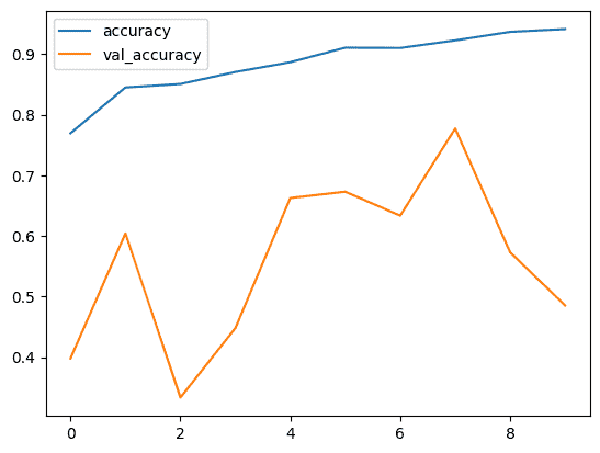
Output

Step 9: Model Evaluation

We evaluate the model using predictions from validation data.

Python `

Y_pred = model.predict(val_data) Y_pred_labels = np.argmax(Y_pred, axis=1) Y_true = val_data.classes from sklearn import metrics

print(metrics.classification_report( Y_true, Y_pred_labels, target_names=classes ))

**Output:

output5

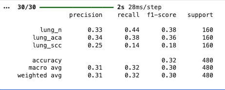
Output

Download full code from here