MiniBatch Gradient Descent in Deep Learning (original) (raw)
Last Updated : 30 Sep, 2025
Mini-batch gradient descent is a variant of the traditional gradient descent algorithm used to optimize the parameters i.e weights and biases of a neural network. It divides the training data into small subsets called mini-batches allowing the model to update its parameters more frequently compared to using the entire dataset at once.
The update rule for Mini-Batch Gradient Descent is:
\theta := \theta - \frac{\alpha}{m} \sum_{i=1}^{m} \nabla_{\theta} \mathcal{L}(\theta; x^{(i)}, y^{(i)})
Where:
- x^{(i)}, y^{(i)} are the input features and labels of the i-th data point in the mini-batch.
- \nabla_{\theta} \mathcal{L}(\theta; x^{(i)}, y^{(i)}) is the gradient of the loss function with respect to \theta for the i-th data point.
Instead of updating weights after calculating the error for each data point (in stochastic gradient descent) or after the entire dataset (in batch gradient descent), mini-batch gradient descent updates the model’s parameters after processing a mini-batch of data. This provides a balance between computational efficiency and convergence stability.
Why to use Mini-Batch Gradient Descent?
The primary reason for using mini-batches is to improve both the computational efficiency and the convergence rate of the training process. By processing smaller subsets of data at a time we can update the weights more frequently than batch gradient descent while avoiding the noisiness of stochastic gradient descent.
It can be summarized as a method that combines the benefits of both batch and stochastic gradient descent:
- Batch gradient descent uses the entire dataset for each iteration which can be computationally expensive.
- Stochastic gradient descent updates the model after each training sample but this can lead to noisy updates and fluctuations in the training process.
Mini-batch gradient descent offers a middle ground making it more efficient and often leading to faster convergence.
How Mini-Batch Gradient Descent Works
- **Splitting the Data: The training dataset is divided into smaller mini-batches. Each mini-batch contains a subset of data points. For example if the dataset has 10,000 examples we might split it into 100 mini-batches each containing 100 data points.
- **Computing the Gradient: For each mini-batch the gradient of the loss function is computed and used to update the model’s parameters. The loss is averaged over the mini-batch which helps in reducing the noise compared to the SGD approach.
- **Updating the Parameters: Once the gradient is computed for a mini-batch the model’s parameters are updated using the learning rate and the gradient. This step is repeated for each mini-batch and the process continues until all mini-batches have been processed.
- **Epochs: An epoch refers to one complete pass through the entire dataset. After each epoch the mini-batches are typically reshuffled to ensure that the model does not overfit to the specific order of the data.
How to Choose the Mini-Batch Size
Choosing the right mini-batch size is crucial for the effectiveness of the model. Here are a few considerations:
- **Small Batch Size: Usually between 32 and 128. This may result in more frequent updates but it can also introduce noise into the optimization process. It is suitable for smaller models or when computational resources are limited.
- **Large Batch Size: Larger than 512. This results in more stable updates but can increase memory consumption. It is ideal when training on powerful hardware like GPUs or TPUs.
- **General Guideline: Start with a batch size of 64 or 128 and adjust based on the training behavior. If training is too slow or unstable then experiment with smaller or larger batch sizes.
Optimizing Mini-Batch Gradient Descent
- **Learning Rate Schedulers: Dynamic adjustment of the learning rate during training can improve the performance of mini-batch gradient descent by helping the model converge more smoothly.
- **Momentum: Using momentum with mini-batch gradient descent can accelerate convergence by helping the model overcome oscillations and reach the global minimum faster.
- **Adam Optimizer: Adam optimizer combines the benefits of both momentum and RMSProp optimizers and is widely used with mini-batch gradient descent for faster and more reliable convergence.
1. Implementing Mini Batch Gradient Descent in TensorFlow
Here mini-batch gradient descent is used by setting batch_size=32 in model.fit() meaning the model processes 32 data points at a time before updating the weights. We are using tensorflow here.
- A custom callback BatchLossHistory is created to track the loss after each mini-batch.
- The on_train_batch_end method captures the loss after each batch
- While on_epoch_begin resets the loss list at the start of each epoch.
- The recorded losses are then plotted to visualize the loss per mini-batch during training. Python `
import tensorflow as tf from tensorflow.keras import layers, models import numpy as np import matplotlib.pyplot as plt
X_train = np.random.rand(1000, 20) y_train = np.random.randint(0, 2, size=(1000, 1))
model = models.Sequential([ layers.Dense(64, activation='relu', input_shape=(20,)), layers.Dense(1, activation='sigmoid') ])
model.compile(optimizer='adam', loss='binary_crossentropy', metrics=['accuracy'])
class BatchLossHistory(tf.keras.callbacks.Callback): def on_train_batch_end(self, batch, logs=None): self.losses.append(logs['loss'])
def on_epoch_begin(self, epoch, logs=None):
    self.losses = []
batch_loss_history = BatchLossHistory()
history = model.fit(X_train, y_train, epochs=10, batch_size=32, callbacks=[batch_loss_history], verbose=1)
plt.plot(batch_loss_history.losses) plt.xlabel('Batch') plt.ylabel('Loss') plt.title('Mini-Batch Loss per Batch') plt.show()
`
**Output:
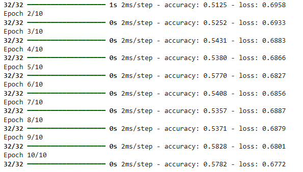
training the model
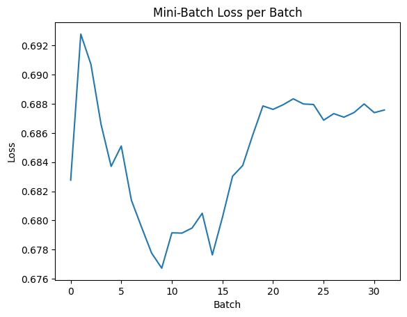
loss-per-batch-tensorflow
2. Implementing Mini Batch Gradient Descent in PyTorch
Here we use PyTorch and set a batch size of 32 set via the DataLoader (batch_size=32). This means that the model processes 32 samples at a time before updating the weights.
- The training loop iterates over mini-batches where the loss for each batch is calculated using the BCELoss function.
- The adam optimizer performs the backward pass and updates the weights.
- Mini-batch loss for each batch is recorded in the batch_losses list.
- After training these losses are plotted to visualize the loss per mini-batch during the 10 epochs. Python `
import torch import torch.nn as nn import torch.optim as optim from torch.utils.data import DataLoader, TensorDataset import matplotlib.pyplot as plt
X_train = torch.randn(1000, 20) y_train = torch.randint(0, 2, (1000, 1)).float()
class SimpleNN(nn.Module): def init(self): super(SimpleNN, self).init() self.fc1 = nn.Linear(20, 64) self.fc2 = nn.Linear(64, 1)
def forward(self, x):
    x = torch.relu(self.fc1(x))
    x = torch.sigmoid(self.fc2(x))
    return x
model = SimpleNN()
criterion = nn.BCELoss() optimizer = optim.Adam(model.parameters(), lr=0.001)
dataset = TensorDataset(X_train, y_train) train_loader = DataLoader(dataset, batch_size=32, shuffle=True)
batch_losses = [] epochs = 10
for epoch in range(epochs): for batch_X, batch_y in train_loader: outputs = model(batch_X) loss = criterion(outputs, batch_y)
    optimizer.zero_grad()
    loss.backward()
    optimizer.step()

    batch_losses.append(loss.item())

print(f"Epoch [{epoch+1}/{epochs}], Loss: {loss.item():.4f}")
plt.plot(batch_losses) plt.xlabel('Batch') plt.ylabel('Loss') plt.title('Mini-Batch Loss per Batch') plt.show()
`
**Output:
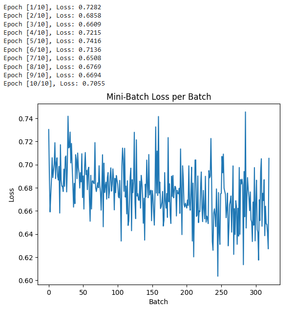
pytorch-mini-batch
Advantages
- **Faster Convergence: Because the model updates its parameters more frequently i.e., after each mini-batch hence converges faster than batch gradient descent which waits until the entire dataset is processed.
- **Reduced Memory Usage: Mini-batches allow training on large datasets without the need to load the entire dataset into memory at once. This makes it feasible to train deep learning models on large-scale data.
- **Smoother Gradient Estimation: Compared to stochastic gradient descent (SGD), mini-batch gradient descent offers a smoother convergence. While SGD updates after each data point resulting in noisy gradients hence mini-batch offers a more balanced and stable gradient update.
- **Parallelization and Speed: It can be parallelized on hardware like GPUs where the computation of gradients for each mini-batch can be executed simultaneously. This results in faster training especially for large neural networks.
Disadvantages
While mini-batch gradient descent is widely used it has a few potential drawbacks:
- **Choice of Batch Size: Selecting the appropriate batch size is crucial. A batch that’s too small may lead to noisy updates, while a batch too large may negate the efficiency benefits.
- **Requires More Epochs: Since it doesn’t use the entire dataset at once it may require more epochs to converge compared to batch gradient descent.
- **Complexity: It introduces complexity in terms of managing multiple mini-batches which can increase the development effort and tuning requirements.