Predict Fuel Efficiency Using Tensorflow in Python (original) (raw)
Last Updated : 23 Jul, 2025
Predicting fuel efficiency is a important task in automotive design and environmental sustainability. In this article we will build a **fuel efficiency prediction model using **TensorFlow one of the most popular deep learning libraries.
We will use the **Auto MPG dataset which contains features like engine displacement, horsepower, weight and other car specifications to predict miles per gallon (MPG).
**Step 1: Import Required Libraries
Before we begin let’s import the necessary libraries: numpy, pandas, matplotlib, seaborn and tensorflow for data processing, model building and visualization.
Python `
import numpy as np import pandas as pd import matplotlib.pyplot as plt import seaborn as sb
import tensorflow as tf from tensorflow import keras from keras import layers
import warnings warnings.filterwarnings('ignore')
`
**Step 2: Load the Dataset
The dataset we’ll use is the **Auto MPG dataset which contains information about cars manufactured between 1970 and 1982. Let’s load the dataset and inspect its structure.
Python `
df = pd.read_csv('auto-mpg.csv') print(df.head())
`
**Output:

Let's check the shape of the data.
Python `
df.shape
`
**Output:
(398, 9)
**Step 3: Exploratory Data Analysis (EDA)
Let’s explore the dataset to understand its structure and identify any inconsistencies.
First we will check the datatypes of the columns using **df.info() function.
Python `
df.info()
`
**Output:
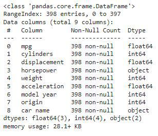
The key information related to dataset are:
- 398 rows of data, with the indices ranging from 0 to 397
- all columns have non-null values, meaning there is no missing data points
- the dataset takes up 28.1 KB of memory
Here, we can observe one discrepancy the horsepower column is given in the object datatype whereas it should be in the numeric datatype.
To understand the numerical characteristics of the dataset, we use **df.describe().
Python `
df.describe()
`
**Output:

Data Cleaning
As per the df.info() part first we will deal with the horsepower column and then we will move toward the analysis part.
Python `
df['horsepower'].unique()
`
**Output:

Here we can observe that instead of the null they have been replaced by the string '?' due to this, the data of this column has been provided in the object datatype.
Python `
print(df.shape) df = df[df['horsepower'] != '?'] print(df.shape)
`
**Output:
(398, 9)
(392, 9)
After this operation, the shape of the dataset decreases from 398 to 392 rows, indicating that we removed 6 rows with invalid values.
Next, we convert the horsepower column to an integer type:
Python `
df['horsepower'] = df['horsepower'].astype(int) df.isnull().sum()
`
**Output:

Python `
df.nunique()
`
**Output:

Visualizing the Impact of Categorical Variables on MPG
Now, let's explore the effect of categorical features like cylinders and origin on the target variable mpg (miles per gallon). We plot bar charts to show the average mpg for different values of cylinders and origin:
Python `
Select only numeric columns for correlation calculation
numeric_df = df.select_dtypes(include=['number'])
plt.subplots(figsize=(15, 5)) for i, col in enumerate(['cylinders', 'origin']): plt.subplot(1, 2, i+1) x = numeric_df.groupby(col).mean()['mpg'] x.plot.bar() plt.xticks(rotation=0) plt.tight_layout() plt.show()
`
**Output:

From this analysis, we observe that the highest mpg values are associated with origin 3 (likely foreign cars).
Correlation Analysis
Next, we explore the relationships between numeric features. We start by plotting the correlation matrix to identify potential multicollinearity issues:
Python `
plt.figure(figsize=(8, 8)) sb.heatmap(numeric_df.corr() > 0.9, annot=True, cbar=False) plt.show()
`
**Output:

If the correlation between two features is too high (i.e., above 0.9), it might cause multicollinearity. In our case, displacement and other features like horsepower and weight might be highly correlated. To address this, we remove displacement using **df.drop():
Python `
df.drop('displacement', axis=1, inplace=True)
`
**Step 4: Data Preprocessing
**Split Data into Features and Target
We now split the dataset into features (independent variables) and target (dependent variable):
Python `
from sklearn.model_selection import train_test_split features = df.drop(['mpg', 'car name'], axis=1) target = df['mpg'].values
X_train, X_val,
Y_train, Y_val = train_test_split(features, target,
test_size=0.2,
random_state=22)
X_train.shape, X_val.shape
`
**Output:
((313, 6), (79, 6))
After splitting, the training set contains 313 rows, and the validation set contains 79 rows.
**Create TensorFlow Data Pipeline
We use TensorFlow to create a data pipeline for efficient training and validation. This involves batching and prefetching the data for better performance:
Python `
AUTO = tf.data.experimental.AUTOTUNE
train_ds = ( tf.data.Dataset .from_tensor_slices((X_train, Y_train)) .batch(32) .prefetch(AUTO) )
val_ds = ( tf.data.Dataset .from_tensor_slices((X_val, Y_val)) .batch(32) .prefetch(AUTO) )
`
**Step 5: Define the Model
We now define the model using **Keras' Sequential API. The model consists of two fully connected layers, each with 256 neurons.
**Batch normalization layers are added for stable and faster training, and a dropout layer is included to prevent overfitting.
Python `
model = keras.Sequential([ layers.Dense(256, activation='relu', input_shape=[6]), layers.BatchNormalization(), layers.Dense(256, activation='relu'), layers.Dropout(0.3), layers.BatchNormalization(), layers.Dense(1, activation='relu') ])
`
Next, we compile the model by specifying the:
- optimizer (adam)
- loss function (mae for Mean Absolute Error)
- evaluation metric (mape for Mean Absolute Percentage Error): Python `
model.compile( loss='mae', optimizer='adam', metrics=['mape'] )
`
Let’s print the summary of the model’s architecture:
Python `
model.summary()
`
**Output:

This shows the number of parameters and the structure of each layer.
Step 6: Model Training
We train the model for 50 epochs using the training and validation datasets. The training process will optimize the model based on the loss and metric we defined earlier:
Python `
history = model.fit(train_ds, epochs=50, validation_data=val_ds)
`
**Output:

**Step 7: Evaluate the Model
After training, we plot the training and validation metrics (loss and mape) to evaluate the model's performance:
Python `
history_df = pd.DataFrame(history.history) history_df.head()
`
**Output:

Python `
history_df.loc[:, ['loss', 'val_loss']].plot() history_df.loc[:, ['mape', 'val_mape']].plot() plt.show()
`
**Output:

After training, we plot the training and validation metrics (loss and mape) to evaluate the model's performance:
**To get source code: **click here
The model consists of dense layers with batch normalization and dropout to prevent overfitting, and it is trained using TensorFlow. The evaluation of the training and validation losses and metrics provides insight into the model's performance.