Spiking Neural Networks in Deep Learning (original) (raw)
Last Updated : 20 May, 2026
Spiking Neural Networks (SNNs) are brain-inspired neural networks that process information using discrete signals called spikes instead of continuous values like traditional neural networks.
- Mimic the behavior of biological neurons
- Use spikes for communication between neurons
- Generate spikes when membrane potential crosses a threshold
- More energy-efficient than traditional neural networks
- Used in pattern recognition and neuromorphic computing
Key Concepts in Spiking Neural Networks
Spiking Neural Networks use biologically inspired mechanisms to process and learn information through spikes and their timing.
1. Neurons and Spikes
Neurons communicate by generating spikes when their membrane potential reaches a threshold.
- Information is transmitted through spikes
- Spike generation depends on membrane potential
- Mimics communication between biological neurons
2. Temporal Coding
In SNNs, the timing of spikes carries important information.
- Uses spike timing to represent information
- Different from traditional rate-based neural networks
- Helps process sequential and time-dependent data
3. Synaptic Weights and Plasticity
Connections between neurons are controlled by synaptic weights, which change during learning.
- Synaptic weights determine spike influence between neurons
- STDP adjusts weights based on spike timing
- Enables learning and adaptation in the network
Working of Spiking Neural Networks
1. Membrane Potential and Firing Threshold
Neurons accumulate incoming spikes in their membrane potential and fire when the threshold is reached.
- Membrane potential stores incoming signal information
- Neurons fire spikes after crossing a threshold
- Potential resets after spike generation
2. Synaptic Integration
Incoming spikes influence connected neurons through weighted synaptic connections.
- Presynaptic spikes affect postsynaptic neurons
- Synaptic weights control spike influence
- Helps propagate information through the network
3. Learning Rules
SNNs learn by adjusting synaptic weights based on spike timing.
- STDP strengthens or weakens synaptic connections
- Earlier presynaptic spikes can strengthen connections
- Enables adaptive and biologically inspired learning
4. Neuron Models
Different neuron models are used to simulate spiking behavior.
- Leaky Integrate-and-Fire (LIF): Simple and widely used neuron model
- Hodgkin-Huxley Model: More biologically realistic neuron model
Implementation of Spiking Neural Network
In this section, we will implement a simple Spiking Neural Network (SNN) using the Leaky Integrate-and-Fire (LIF) neuron model for detecting a specific spike pattern.
Step 1: Define Neuron and Synapse Classes
- The
LIFNeuronclass models the behavior of a leaky integrate-and-fire neuron. - The
Synapseclass represents the connection between neurons with an associated weight. Python `
import numpy as np
class LIFNeuron: def init(self, threshold, reset_value, decay_factor, refractory_period): self.threshold = threshold self.reset_value = reset_value self.decay_factor = decay_factor self.refractory_period = refractory_period self.membrane_potential = 0 self.spike_time = -1 self.refractory_end_time = -1
def update(self, incoming_spikes, current_time):
    if current_time < self.refractory_end_time:
        return False

    self.membrane_potential *= self.decay_factor
    self.membrane_potential += np.sum(incoming_spikes)

    if self.membrane_potential >= self.threshold:
        self.spike_time = current_time
        self.membrane_potential = self.reset_value
        self.refractory_end_time = current_time + self.refractory_period
        return True
    return False
class Synapse: def init(self, weight): self.weight = weight
`
Step 2: Define the STDP Learning Rule
The stdp function adjusts the synaptic weights based on the timing difference between the pre- and post-synaptic spikes.
Python `
def stdp(pre_spike_time, post_spike_time, weight, learning_rate, tau_positive, tau_negative): if pre_spike_time > 0 and post_spike_time > 0: delta_t = post_spike_time - pre_spike_time if delta_t > 0: return weight + learning_rate * np.exp(-delta_t / tau_positive) else: return weight - learning_rate * np.exp(delta_t / tau_negative) return weight
`
Step 3: Initialize Simulation Parameters and Network
- Set the number of time steps and the sizes of input, hidden, and output layers.
- Initialize neurons and synapses with their parameters and random weights. Python `
time_steps = 100 input_size = 5 hidden_size = 3 output_size = 1
input_neurons = [LIFNeuron(threshold=1.0, reset_value=0.0, decay_factor=0.9, refractory_period=2) for _ in range(input_size)] hidden_neurons = [LIFNeuron(threshold=1.0, reset_value=0.0, decay_factor=0.9, refractory_period=2) for _ in range(hidden_size)] output_neurons = [LIFNeuron(threshold=1.0, reset_value=0.0, decay_factor=0.9, refractory_period=2) for _ in range(output_size)]
input_to_hidden_synapses = np.random.rand(input_size, hidden_size) hidden_to_output_synapses = np.random.rand(hidden_size, output_size)
learning_rate = 0.01 tau_positive = 20 tau_negative = 20
`
Step 4: Define the Spike Train Pattern to Detect
Set the pattern of spikes that the network should detect.
Python `
pattern = [1, 0, 1, 0, 1]
`
Step 5: Simulation Loop
- Run the simulation for the defined number of time steps.
- Update neurons and synapses at each time step.
- Apply the STDP learning rule to adjust synaptic weights.
- Check if the pattern is detected. Python `
for t in range(time_steps): input_spikes = np.random.randint(0, 2, size=input_size)
hidden_spikes = np.zeros(hidden_size)
for i, neuron in enumerate(input_neurons):
    if neuron.update(input_spikes[i] * input_to_hidden_synapses[i], t):
        hidden_spikes += input_to_hidden_synapses[i]

output_spikes = np.zeros(output_size)
for j, neuron in enumerate(hidden_neurons):
    if neuron.update(hidden_spikes[j] * hidden_to_output_synapses[j], t):
        output_spikes += hidden_to_output_synapses[j]

for k, neuron in enumerate(output_neurons):
    neuron.update(output_spikes[k], t)

for i in range(input_size):
    for j in range(hidden_size):
        input_to_hidden_synapses[i, j] = stdp(input_neurons[i].spike_time, hidden_neurons[j].spike_time, input_to_hidden_synapses[i, j], learning_rate, tau_positive, tau_negative)
for j in range(hidden_size):
    for k in range(output_size):
        hidden_to_output_synapses[j, k] = stdp(hidden_neurons[j].spike_time, output_neurons[k].spike_time, hidden_to_output_synapses[j, k], learning_rate, tau_positive, tau_negative)

if all(neuron.spike_time == t for neuron, pat in zip(input_neurons, pattern) if pat == 1):
    print(f"Pattern detected at time step {t}")
`
**Output:
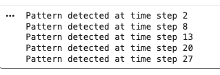
Output
Download full code from here
Applications
- Used in neuromorphic computing for energy-efficient hardware
- Applied in robotics for real-time sensory processing and control
- Supports autonomous navigation and adaptive robotic behavior
- Used in Brain-Computer Interfaces (BCIs) to decode neural signals
- Helps control prosthetic and external devices using brain activity
Challenges
- Training is difficult due to discrete spike-based computations
- Traditional backpropagation cannot be directly applied
- Requires advanced methods like surrogate gradients and ANN-to-SNN conversion
- Large-scale SNN simulations demand high computational resources
- Specialized neuromorphic hardware is often needed for efficient execution