Softmax Activation Function in Neural Networks (original) (raw)
Last Updated : 17 Nov, 2025
In Deep Learning, activation functions are important because they introduce non-linearity into neural networks allowing them to learn complex patterns. Softmax Activation Function transforms a vector of numbers into a probability distribution, where each value represents the likelihood of a particular class. It is especially important for multi-class classification problems.
- Each output value lies between 0 and 1.
- The sum of all output values equals 1.
This property makes Softmax ideal for scenarios where each output neuron represents the probability of a distinct class.
Softmax Function
For a given vector, z = [z_1, z_2, \dots, z_n]the Softmax function is defined as:
\sigma(z_i) = \frac{e^{z_i}}{\sum_{j=1}^{n} e^{z_j}}
**where:
- e^{z_j}: Exponentiation of the input value.
- \sum_{j=1}^{n} e^{z_j}: Sum of all exponentiated values to normalize outputs.
Each output \sigma(z_i) represents the probability of class i.
Key Characteristics
- **Normalization: Converts logits into a probability distribution where the sum equals 1.
- **Exponentiation: Amplifies larger values making the model’s confidence more pronounced.
- **Differentiable: Enables gradient-based optimization during backpropagation.
- **Probabilistic Interpretation: Makes output easier to interpret as class likelihoods.
How Softmax Activation Function Works
Softmax converts a vector of raw scores into a probability distribution.
- **Input Scores: Take the raw output vector from the model. These values can be any real numbers.
- **Exponentiate: Apply e^x to make every value positive and amplify differences.
- **Sum of exponentials: Compute the normalising constant Z = \sum e^{x'}
- **Normalize: Divide each exponent by Z to get probabilities p_i = \frac{e^{x'_i}}{Z}.
- **Output (Probabilities): Final probability vector can be used with argmax to pick the predicted class.
Step-By-Step Implementation
Step 1: Import Necessary Libraries
- Import NumPy for numerical operations
- TensorFlow and Keras to build and train the neural network
- Use Matplotlib for visualizing training accuracy and loss. Python `
import numpy as np import tensorflow as tf from tensorflow.keras.models import Sequential from tensorflow.keras.layers import Dense from tensorflow.keras.utils import to_categorical from sklearn.datasets import load_iris from sklearn.model_selection import train_test_split import matplotlib.pyplot as plt
`
Step 2: Load and Prepare the Dataset
- Load the Iris dataset multi-class classification dataset.
- Extract features and labels from the dataset.
- Convert labels to one-hot encoded format for softmax based training.
- Split the data into training and testing sets for evaluation. Python `
iris = load_iris()
X = iris.data
y = iris.target
y_encoded = to_categorical(y)
X_train, X_test, y_train, y_test = train_test_split(X, y_encoded, test_size=0.2, random_state=42)
`
Step 3: Neural Network Model
- Sequential to create a simple feedforward neural network.
- The hidden layer uses ReLU activation to learn non linear patterns.
- The output layer uses Softmax activation to produce class probabilities. Python `
model = Sequential([
Dense(8, input_shape=(4,), activation='relu'),
Dense(3, activation='softmax')
])
`
Step 4: Compile the Model
- Define Adam optimizer for efficient gradient updates.
- categorical_crossentropy as the loss function for multi-class problems.
- Compiling prepares the model for training. Python `
model.compile(optimizer='adam', loss='categorical_crossentropy', metrics=['accuracy'])
`
Step 5: Train the Model
- Train the model using the training dataset.
- Run for 100 epochs with a small batch size for better learning.
- Use validation_split=0.2 to monitor overfitting during training.
- The history object stores loss and accuracy data for visualization Python `
history = model.fit(X_train, y_train, epochs=100, batch_size=8, validation_split=0.2, verbose=0)
`
Step 6: Predict and Display Probabilities
- Use the trained model to predict class probabilities via Softmax.
- Determine the predicted class with the highest probability.
- Display both predicted probabilities and the corresponding class name. Python `
sample = np.array([[5.1, 3.5, 1.4, 0.2]])
prediction = model.predict(sample)
predicted_class = np.argmax(prediction)
print("\nPredicted Probabilities (Softmax Output):", prediction) print("Predicted Class:", iris.target_names[predicted_class])
`
**Output:
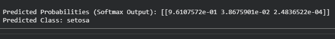
Prediction
You can download full code from here.
Why Use Softmax in the Last Layer
The Softmax Activation function is typically used in the final layer of a classification neural network because:
- It transforms the model raw output into interpretable probabilities.
- It ensures the outputs are mutually exclusive suitable for problems where each sample belongs to exactly one class.
- It works seamlessly with the Cross Entropy Loss Function which measures the difference between predicted and actual probabilities.
Applications
- **Neural Networks: Used in the output layer of models like CNNs or MLPs for multi-class classification.
- **Attention Mechanisms: Assigns attention weights to different tokens or words, normalizing them to sum to 1.
- **Reinforcement Learning: Converts Q values or action values into probabilities for stochastic action selection.
- **Model Ensembles: Combines multiple model predictions into a single probabilistic output.
Challenges
- **Overconfidence: Tends to produce extremely confident predictions even for uncertain inputs.
- **Sensitivity to Outliers: Small variations in logits can cause large shifts in probability outputs.
- **Softmax Bottleneck: Limited ability to model complex relationships between output classes.
- **Poor Calibration: Predicted probabilities often do not align with true likelihoods.
- **Gradient Saturation: Can cause vanishing gradients when one class probability dominates others.
Difference Between Sigmoid and Softmax Activation Function
Sigmoid and Softmax are activation functions used in classification tasks.
- Sigmoid gives a single probability for binary output.
- Softmax distributes probabilities across multiple classes in multi-class problems.
| Parameters | Sigmoid Activation Function | Softmax Activation Function |
|---|---|---|
| Definition | Maps any real valued input to a value between 0 and 1 | Converts a vector of real number into a probability distribution |
| Purpose | Used for binary classification problems | Used for multi class classification problems |
| Number of Outputs | one independent probability per neuron | Multiple interdependent probabilities for all classes |
| Use Case | Predicting two classes | Predicting multiple classes |
| Output | Represents confidence for one class | Represents probabilities for all classes |
Applications
- **Neural Networks: Used in the output layer of models like CNNs or MLPs for multi-class classification.
- **Attention Mechanisms: Assigns attention weights to different tokens or words, normalizing them to sum to 1.
- **Reinforcement Learning: Converts Q values or action values into probabilities for stochastic action selection.
- **Model Ensembles: Combines multiple model predictions into a single probabilistic output.
Challenges
- **Overconfidence: Tends to produce extremely confident predictions even for uncertain inputs.
- **Sensitivity to Outliers: Small variations in logits can cause large shifts in probability outputs.
- **Softmax Bottleneck: Limited ability to model complex relationships between output classes.
- **Poor Calibration: Predicted probabilities often do not align with true likelihoods.
- **Gradient Saturation: Can cause vanishing gradients when one class probability dominates others.