Wasserstein Generative Adversarial Networks (WGANs) (original) (raw)
Last Updated : 23 Jul, 2025
Wasserstein Generative Adversarial Network (WGANs) is a variation of Deep Learning GAN with little modification in the algorithm. Generative Adversarial Network (GAN) is a method for constructing an efficient generative model. Martin Arjovsky, Soumith Chintala, and Léon Bottou developed this network in 2017. This is used widely to produce real images.
Wasserstein Generative Adversarial Network
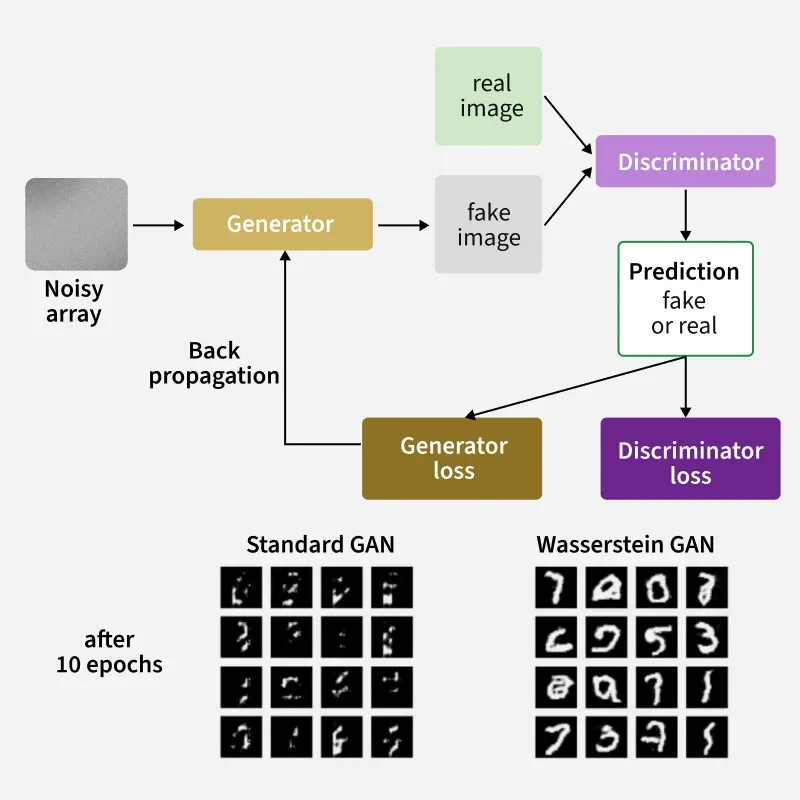
WGAN's architecture uses deep neural networks for both generator and discriminator. The key difference between GANs and WGANs is the loss function and the gradient penalty. WGANs were introduced as the solution to mode collapse issues. The network uses the Wasserstein distance, which provides a meaningful and smoother measure of distance between distributions.
WGAN architecture
WGANs use the Wasserstein distance, which provides a more meaningful and smoother measure of distance between distributions.
W(\mathbb{P}_r , \mathbb{P}_g) = \inf_{\gamma \epsilon \prod (\mathbb{P}_r,\mathbb{P}_g )}\mathbb{E}_{(x,y)\sim \gamma)}\left [ ||x-y|| \right ]
- γ denotes the mass transported from x to y in order to transform the distribution Pr to Pg.
- denotes the set of all joint distributions γ(x, y) whose marginals are respectively Pr and Pg.
The benefit of having Wasserstein Distance instead of Jensen-Shannon (JS) or Kullback-Leibler divergence is as follows:
- W (Pr, Pg) is continuous.
- W (Pr, Pg) is differential everywhere.
- Whereas Jensen-Shannon divergence and other divergence or variance are not continuous, but rather discrete.
- Hence, we can perform gradient descent and we can minimize the cost function.
Wasserstein GAN Algorithm
The algorithm is stated as follows:
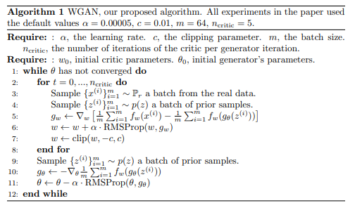
- The function f solves the maximization problem given by the Kantorovich-Rubinstein duality. To approximate it, a neural network is trained parametrized with weights w lying in a compact space W and then backprop as a typical GAN.
- To have parameters w lie in a compact space, we clamp the weights to a fixed box. Weight clipping is although terrible, yields good results when experimenting. It is simpler and hence implemented. EM distance is continuous and differentiable allows to train the critic till optimality.
- The JS gradient is stuck at local minima but the constrain of weight limits allows the possible growth of the function to be linear in most parts and get optimal critic.
- Since the optimal generator for a fixed discriminator is a sum of deltas on the places the discriminator assigns the greatest values to, we train the critic until optimality prevents modes from collapsing.
- It is obvious that the loss function at this stage is an estimate of the EM distance, as the critic f in the for loop lines indicates, prior to each generator update. Thus, it makes it possible for GAN literature to correlate based on the generated samples' visual quality.
- This makes it very convenient to identify failure modes and learn which models perform better than others without having to look at the generated samples.
Benefits of WGAN algorithm over GAN
- WGAN is more stable due to the Wasserstein Distance which is continuous and differentiable everywhere allowing to perform gradient descent.
- It allows to train the critic till optimality.
- There is still no evidence of model collapse.
- Not struck in local minima in gradient descent.
- WGANs provide more flexibility in the choice of network architectures. The weight clipping, generators architectures can be changed according to choose.
Generating Images using WGANs
The steps to generate images using WGANS are discussed below:
Step 1: Import the required libraries
For the implementation, required python libraries are: numpy, keras, matplotlib.
Python `
from numpy import expand_dims from numpy import mean from numpy import ones from numpy.random import randn from numpy.random import randint from keras.datasets.mnist import load_data from keras import backend from keras.optimizers import RMSprop from keras.models import Sequential from keras.layers import Dense from keras.layers import Reshape from keras.layers import Flatten from keras.layers import Conv2D from keras.layers import Conv2DTranspose from keras.layers import LeakyReLU from keras.layers import BatchNormalization from keras.initializers import RandomNormal from keras.constraints import Constraint from matplotlib import pyplot import tensorflow as tf
`
Step 2: Define wasserstein loss function
To define the wasserstein loss function, we use the following method. Our goal is to minimize the Wasserstein distance between distribution of generated samples and distribution of real samples. The following is an efficient implementation of wasserstein loss function where the score is maximum. We take the average distance, so we use backend.mean()
Python `
def wasserstein_loss(y_true, y_pred): return tf.reduce_mean(y_true * y_pred) # Use tf.reduce_mean() instead of K.mean() or backend.mean()
`
Step 3: Generate images
First is we need to generate the images from the dataset as follows: We will be using the class of digit 5, we can use any value.
Python `
def load_real_samples(): (trainX, trainy), (_, _) = load_data() selected_ix = trainy == 5 X = trainX[selected_ix] X = expand_dims(X, axis=-1) X = X.astype('float32') X = (X - 127.5) / 127.5 return X
select real samples
def generate_real_samples(dataset, n_samples): ix = randint(0, dataset.shape[0], n_samples) X = dataset[ix] y = -ones((n_samples, 1)) return X, y
`
Step 4: Generate Samples
Randomly we need to generate real samples from the dataset above we chosen as X.
Python `
def generate_real_samples(dataset, n_samples): ix = randint(0, dataset.shape[0], n_samples) X = dataset[ix] y = -ones((n_samples, 1)) return X, y
`
Step 5: Define Critic and Discriminator Model
It is the time to define the critic or discriminator model. We need to update the discriminator model more than generator since it needs to be more accurate otherwise the generator will easily make it fool. Before that, we need the clip constraint to be applied on our weights since we discussed we need the gradient descent and hence we make it cubic clip.
Python `
clip model
class ClipConstraint(Constraint): def init(self, clip_value): self.clip_value = clip_value def call(self, weights): return backend.clip(weights, -self.clip_value, self.clip_value)
`
And then we define the critic
Python `
def define_critic(in_shape=(28,28,1)): init = RandomNormal(stddev=0.02) const = ClipConstraint(0.01) model = Sequential() model.add(Conv2D(64, (4,4), strides=(2,2), padding='same', kernel_initializer=init, kernel_constraint=const, input_shape=in_shape)) model.add(BatchNormalization()) model.add(LeakyReLU(alpha=0.2)) model.add(Conv2D(64, (4,4), strides=(2,2), padding='same', kernel_initializer=init, kernel_constraint=const)) model.add(BatchNormalization()) model.add(LeakyReLU(alpha=0.2)) model.add(Flatten()) model.add(Dense(1)) opt = RMSprop(learning_rate=0.00005) model.compile(loss=wasserstein_loss, optimizer=opt) return model
`
Step 6: Define Generator Model
In the generator model, we simply take a 28x28 image and downscale it to 7x7 for better performance and model it accurately.
Python `
def define_generator(latent_dim):
init = RandomNormal(stddev=0.03)
model = Sequential()
n_nodes = 128 * 7 * 7
model.add(Dense(n_nodes, kernel_initializer=init, input_dim=latent_dim))
model.add(LeakyReLU(alpha=0.2))
model.add(Reshape((7, 7, 128)))
model.add(Conv2DTranspose(128, (4,4), strides=(2,2), padding='same', kernel_initializer=init))
model.add(BatchNormalization())
model.add(LeakyReLU(alpha=0.2))
model.add(Conv2DTranspose(128, (4,4), strides=(2,2), padding='same', kernel_initializer=init))
model.add(BatchNormalization())
model.add(LeakyReLU(alpha=0.2))
model.add(Conv2D(1, (7,7), activation='tanh', padding='same', kernel_initializer=init))
return model
`
Step 7: Update the generator
The following method is used to update the generator in GAN. We use the Root Mean Square as our optimizer for the generator since the Adam optimizer generates problem for the model.
Python `
def define_gan(generator, critic): # make weights in the critic not trainable for layer in critic.layers: if not isinstance(layer, BatchNormalization): layer.trainable = False model = Sequential() model.add(generator) model.add(critic) opt = RMSprop(learning_rate=0.00005) model.compile(loss=wasserstein_loss, optimizer=opt) return model
`
Step 8: Generate Fake Samples
Now to generate fake samples, we need latent space, so we put take the latent space and the number of samples and then ask the generator to predict the samples.
Python `
def generate_latent_points(latent_dim, n_samples): x_input = randn(latent_dim * n_samples) x_input = x_input.reshape(n_samples, latent_dim) return x_input
fake examples
def generate_fake_samples(generator, latent_dim, n_samples): x_input = generate_latent_points(latent_dim, n_samples) X = generator.predict(x_input) y = ones((n_samples, 1)) return X, y
`
Step 9: Model Training
It is the time to train the model. Remember we update the critic/discrimnator more than the generator to make it flawless. You can check the generated image in the directory.
Python `
train the generator and critic
def train(g_model, c_model, gan_model, dataset, latent_dim, n_epochs=10, n_batch=64, n_critic=5):
bat_per_epo = int(dataset.shape[0] / n_batch)
# number of training iterations
n_steps = bat_per_epo * n_epochs
half_batch = int(n_batch / 2)

c1_hist, c2_hist, g_hist = list(), list(), list()

for i in range(n_steps):
    # update the critic
    c1_tmp, c2_tmp = list(), list()
    for _ in range(n_critic):
        X_real, y_real = generate_real_samples(dataset, half_batch)
        c_loss1 = c_model.train_on_batch(X_real, y_real)
        c1_tmp.append(c_loss1)
        X_fake, y_fake = generate_fake_samples(g_model, latent_dim, half_batch)
        c_loss2 = c_model.train_on_batch(X_fake, y_fake)
        c2_tmp.append(c_loss2)
    c1_hist.append(mean(c1_tmp))
    c2_hist.append(mean(c2_tmp))
    X_gan = generate_latent_points(latent_dim, n_batch)
    y_gan = -ones((n_batch, 1))
    g_loss = gan_model.train_on_batch(X_gan, y_gan)
    g_hist.append(g_loss)
    print('>%d, c1=%.3f, c2=%.3f g=%.3f' % (i+1, c1_hist[-1], c2_hist[-1], g_loss))
    if (i+1) % bat_per_epo == 0:
        summarize_performance(i, g_model, latent_dim)
# line plots of loss
plot_history(c1_hist, c2_hist, g_hist)
`
Step 10: Visualization
We use the following plot functions. You can check the history plot in your directory.
Python `
def summarize_performance(step, g_model, latent_dim, n_samples=100): X, _ = generate_fake_samples(g_model, latent_dim, n_samples) X = (X + 1) / 2.0 for i in range(10 * 10): pyplot.subplot(10, 10, 1 + i) pyplot.axis('off') pyplot.imshow(X[i, :, :, 0], cmap='gray_r') filename1 = 'plot_%04d.png' % (step+1) pyplot.savefig(filename1) pyplot.close()
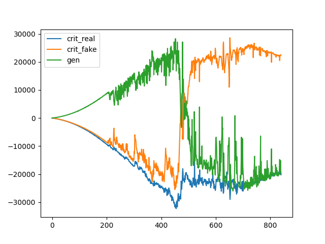
def plot_history(d1_hist, d2_hist, g_hist): pyplot.plot(d1_hist, label='crit_real') pyplot.plot(d2_hist, label='crit_fake') pyplot.plot(g_hist, label='gen') pyplot.legend() pyplot.savefig('line_plot_loss.png') pyplot.close()
`
Now to test it run it as follows:
Python `
latent_dim = 50 critic = define_critic() generator = define_generator(latent_dim) gan_model = define_gan(generator, critic) dataset = load_real_samples() print(dataset.shape) train(generator, critic, gan_model, dataset, latent_dim)
`
**Output:
11490434/11490434 [==============================] - 0s 0us/step
(5421, 28, 28, 1)
1/1 [==============================] - 1s 882ms/step
1/1 [==============================] - 0s 106ms/step
1/1 [==============================] - 0s 50ms/step
1/1 [==============================] - 0s 25ms/step
1/1 [==============================] - 0s 36ms/step
>1, c1=-13.690, c2=-4.848 g=18.497
1/1 [==============================] - 0s 24ms/step
1/1 [==============================] - 0s 23ms/step
1/1 [==============================] - 0s 44ms/step
1/1 [==============================] - 0s 24ms/step
1/1 [==============================] - 0s 33ms/step
>2, c1=-28.276, c2=0.991 g=16.891
1/1 [==============================] - 0s 57ms/step
1/1 [==============================] - 0s 33ms/step
1/1 [==============================] - 0s 70ms/step
1/1 [==============================] - 0s 113ms/step
1/1 [==============================] - 0s 49ms/step
>3, c1=-39.209, c2=-34.840 g=22.131
The samples generated by our GAN model. We can merge the plots as follows:
Python `
import os import imageio
imgdir = '/content/'
List all files starting with 'plot_'
gif_files = [file for file in os.listdir(imgdir) if file.startswith('plot_')] gif_files.sort()
images = [] for image_file in gif_files: image_path = os.path.join(imgdir, image_file) images.append(imageio.imread(image_path))
Save the images as a GIF
imageio.mimsave('/content/output.gif', images, format="GIF", fps=2)
`
**Output:
As we see, before the epoch 300, we have very unclear generation, and it doesn't correlates to digit 5. But after that, we see some good generation of fake digits which appears real. Hence, we see clearer images as we progress. At the starting stage, the generator gets adjusted to compete with discriminator and provides initialized data modified slightly. After running several epochs, generator gets adjusted and produces good results.
**And the loss graph is as follows:
**Related Article: