Introduction to Amortized Analysis (original) (raw)
Last Updated : 25 Feb, 2026
Amortized analysis studies the average cost of operations over a sequence, rather than focusing on the worst-case of a single operation.
- It is especially useful for dynamic data structures like arrays, hash tables, and trees, where occasional expensive operations occur.
- By spreading the cost of rare costly operations across many cheap ones, it gives a realistic measure of algorithm efficiency.
**Example: In a dynamic array, inserting elements is usually cheap (O(1)), but occasionally the array needs resizing, which is costly. By spreading the cost of resizing over all insertions, the amortized cost per insertion remains O(1).
Techniques of Amortized Analysis
There are three standard methods to perform amortized analysis:
**1. Aggregate Method
- Compute the total cost of 𝑛n operations and divide it by number of operations to obtain the average cost..
- Example: Dynamic array insertions involve occasional costly resizes, but the average cost per insertion is low.
**2. Accounting Method
- Assign credits to operations.
- Cheap operations save credits to pay for future expensive operations.
**3. Potential Method
- Define a potential function φ representing the “stored work” in a data structure.
- Amortized cost = actual cost + change in potential.
- Commonly used in balanced trees like Red-Black Trees.
Amortized Analysis of Dynamic Sized Array Insertions
When designing a dynamic sized array (vector in C++, list in Python and ArrayList in Java), we must decide on the size. There is a trade-off between space and time. If the size is large, we waste space.
The solution is to increase the table size whenever it's full. Here are the steps:
- Allocate memory for a larger table, typically twice the size of the old table.
- Copy the contents of the old table to the new table.
- Free the old table.
If space is available, insert a new item.
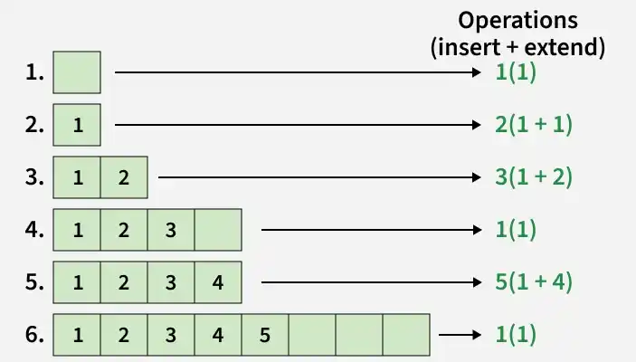
**Time Complexity: If simple analysis is used, the worst-case insertion cost is O(n). Therefore, the worst-case cost for n insertions is n * O(n), which is O(n^2). However, this analysis provides an upper bound that isn't tight for n insertions, as not all insertions take O(n) time.
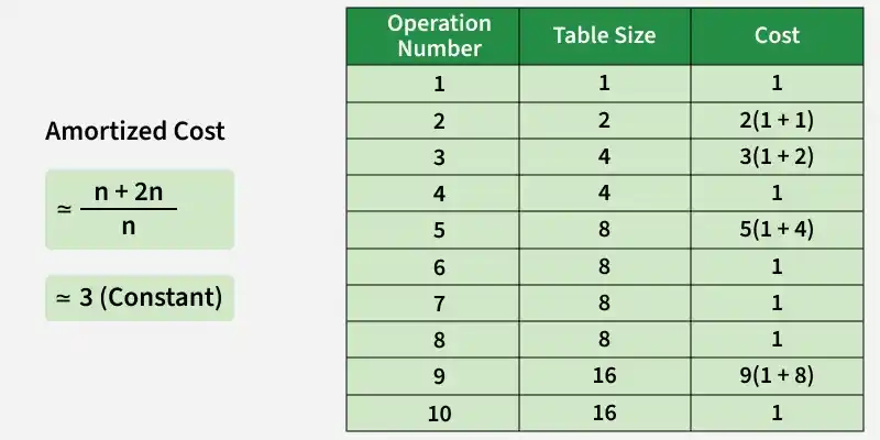
Amortized Analysis proves the Dynamic Table scheme has O(1) insertion time, vital in hashing.
**Note: Amortized Analysis doesn't involve probability. Randomized Analysis analyzes algorithms using randomization, such as Randomized Quick Sort, Quick Select, and Hashing.
Amortized Analysis of Insertion in a Red-Black Tree
Amortized analysis of Red-Black Tree insertions uses the Potential Method, where a new node is inserted at a leaf. A potential function φ assigns a non-negative value to the tree, and each operation may change this potential to calculate the amortized cost.
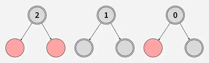
Let us define the potential function φ:
g(n) = 0, if n is red.
1, if n is black with no red children.
0, if n is black with one red child.
2, if n is black and has two red children.
where n is a node of the Red-Black Tree. The potential function φ = ∑ g(n), over all nodes.
Amortized time = c + Δφ(h)
Δφ(h) = φ(h') - φ(h)
where h and h' are the states before and after the operation, respectively, and c is the actual cost.
The change in potential should be positive for low-cost operations and negative for high-cost operations.
The insertions and their amortized analysis can be represented as:
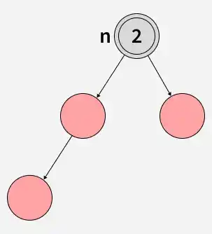
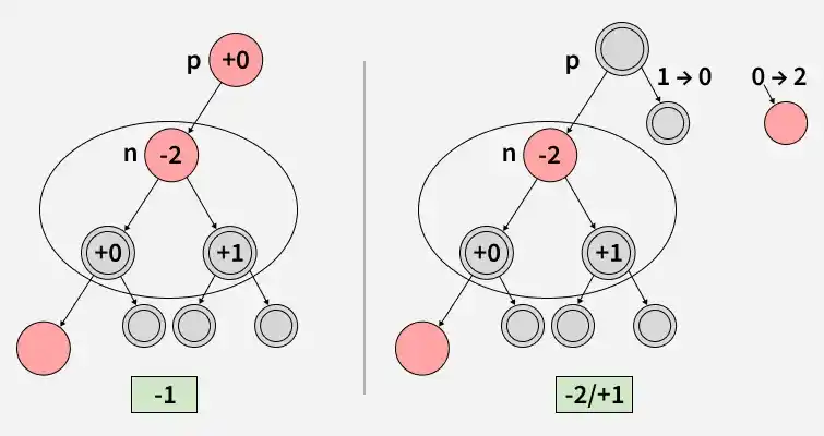
This insertion starts by recoloring the parent and sibling. Then, the grandparent and uncle are considered, resulting in amortized costs of -1 (red grandparent), -2 (black uncle and grandparent), or +1 (red uncle and black grandparent). The insertion can be shown as:
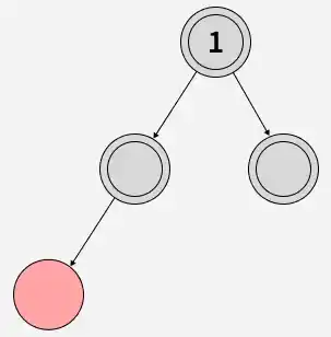
In this insertion, the node is inserted without changes because the black depth remains the same. This occurs when the leaf has a black sibling or no sibling, as the null node is black.
So, the amortized cost of this insertion is 0.
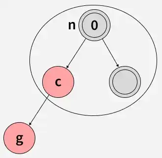
In this insertion, we cannot recolor the leaf node, its parent, and the sibling such that the black depth stays the same as before. So, we need to perform a Left- Left rotation.
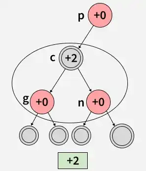
After rotation, no changes occur when the grandparent is black or red. The insertion is completed with an amortized cost of +2, as shown below:
After calculating amortized costs at the leaf level, we can analyze the overall insertion cost.
- In some cases, a chain of red parent-child relationships may extend to the root.
- In the worst-case, the number of black nodes with two red children decreases by at most 1, while the number of black nodes with no red children increases by at most 1.
This results in a net loss of at most 1 in the potential function.
Since each unit of potential compensates for one operation, we conclude that: Δφ(h) ≤ n, where n represents the total number of nodes in the Red-Black Tree.
Applications
Amortized Analysis is useful for designing efficient algorithms for data structures such as:
- Dynamic Arrays
- Priority Queues
- Disjoint-Set Data Structures and many more.