Block Diagram Reduction Rules (original) (raw)

Last Updated : 10 Mar, 2026

A complex control system is difficult to analyze as various factors are associated with it. In this article, we will see how to easily analyze a control system, and this is only possible by using block diagram reduction rules. This representation of a system involves summing points, functional blocks, etc., connected through branches, which makes the analysis easy, simple, and step-by-step, crystal clear.

Methods of Block Diagram Reduction Rules

In a Control system, for the analysis of any system, there are two methods

1. Transfer Function Approach
2. State Variable Approach

**Transfer Function Approach: The ratio of the Laplace transform of the output variable to the Laplace transform of the input variable, assuming all the initial conditions to be zero, is called the transfer function.

**State Variable Approach: The advantage of the Transfer Function Approach is that it gives a simple mathematical algebraic equation, and it directly gives poles and zeroes of the system. The stability of the system and output of the system for any input can be directly determined from this approach.

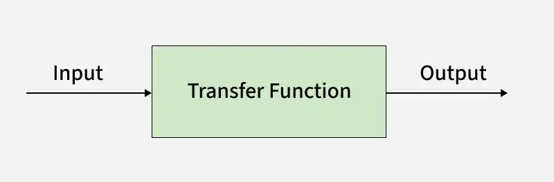
Transfer Function Block Diagram

Transfer Function G(s) = \frac{\mathcal{L}\{c(t)\}}{\mathcal{L}\{r(t)\}} all the initial conditions are zeroes.

G(s) = \frac{C(s)}{R(s)}

It is not always convenient to determine the complete transfer function for the very complex control system. Therefore function of each element of the control system is depicted in the form of a block diagram.

The symbol representation in short form gives a relation of output to input in the control system. The complete system can be formed by connecting each block as per the need of the system.

Block Diagram Reduction Rules

To form a control system the block are arranged together as required and the steps followed to obtain the transfer function are called Block Diagram Reduction Method.

Following are the rules to be followed during finding the transfer function of the system

**Rule 1 : when more than one block is cascaded than overall transfer function is multiplication of all the transfer function .

\begin{aligned}G_1(s) &= \frac{C_1(s)}{R(s)} \\G_2(s) &= \frac{C_2(s)}{C_1(s)} \\G_3(s) &= \frac{C(s)}{C_2(s)}\end{aligned}

\frac{C(s)}{R(s)} = G_1(s) \cdot G_2(s) \cdot G_3(s)

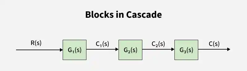
Blocks in cascade

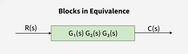
Blocks in Equivalence

**Rule 2 : When two or more input signal enters into system that point is known as Summing Point and the output coming out from summing point will be the sum of all the input entered through summing point .

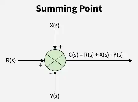
Summing Point

**Rule 3 : When there are two or more summing point than we can change the position of summing point with each other as shown below in figure.

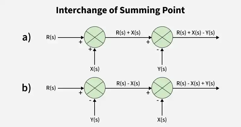
Interchange of summing point

**Rule 4 : When one or more blocks are connected in parallel to other block than the final equivalent transfer function can be find as following

C(s) = R(s)G_1(s) + R(s)G_2(s) + R(s)G_3(s)

C(s) = R(s) \left[ G_1(s) + G_2(s) + G_3(s) \right]

\frac{C(s)}{R(s)} = G_1(s) + G_2(s) + G_3(s)

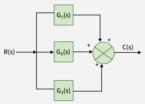
Blocks in Parallel

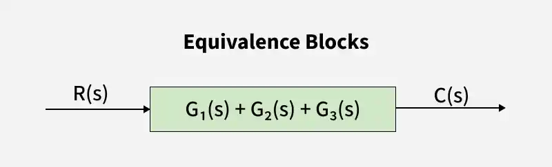
Equivalence Blocks

**Rule 5 : When take off point is shifted from position before block to a position after block than a block is added having gain equals to reciprocal of current gain as shown below.

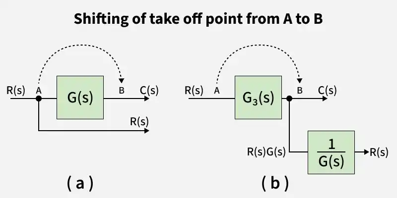
Shifting of Take-off Point from A to B

**Rule 6 : When take off point is shifted from a position after block to a position before the block than a block is added having gain equals to current gain as shown below .

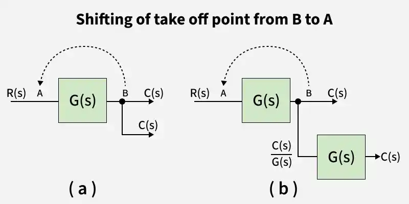
Shifting the off point from B to A

**Rule 7 : When a summing point is shifted from a position before a block to position after the block , a block is added to summing point having gain equals to current gain.

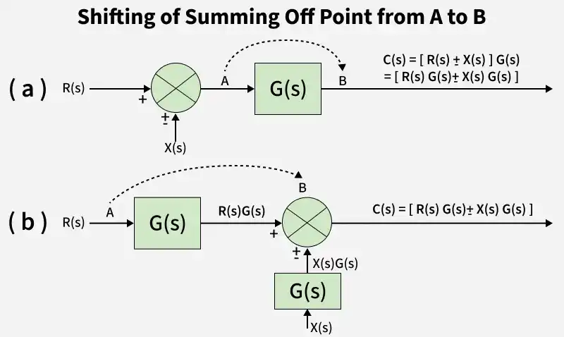
Shifting of Summing Point from A to B

**Rule 8 : When a summing point is shifted from a position after a block to a position before the block , a block is added having gain equals to reciprocal of current gain .

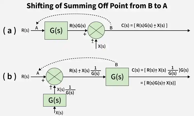
Shifting of Summing Point from B to A

**Rule 9 : when a take off point is shifted from a position before a summing point to position after the summing point , it takes place as shown in below figure.

Shifting of Take-off Point before summing point to after Summing Point

**Rule 10 : Shifting a take off point from a position after a summing point to position before summing point is shown in below figure.

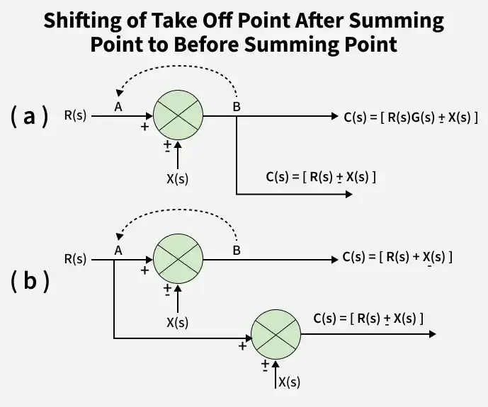
Shifting of Take-off Point after Summing Point to before Summing Point

**Rule 11 : Elimination of summing point in closed loop system is done as shown in below figure.

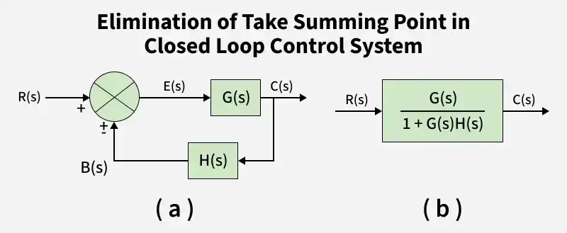
Elimination of the Summing Point in Closed Loop Control System

Advantages

• Simplifies the representation of complex control systems using clear block structures.
• Allows performance analysis of each block separately.
• Helps in determining the transfer function of a control system easily.
• Makes stability analysis easier by observing the feedback path.
• Provides a clear view of the functional operation of the system.

Disadvantages

• Reduction process becomes time-consuming for very complex systems.
• Some internal functional details may disappear during simplification.
• Does not represent the physical construction of the system.
• Provides no information about the energy source used in the system.

Applications

• Used in hardware system design.
• Applied in electrical system modeling and analysis.
• Useful in software system structure design.
• Used in process flow representation.
• Helps in determining the transfer function of a system.
• Assists in analyzing system stability.

Solved Problems on Block Diagram Reduction

**Reduce the following block diagram using the block diagram reduction rule

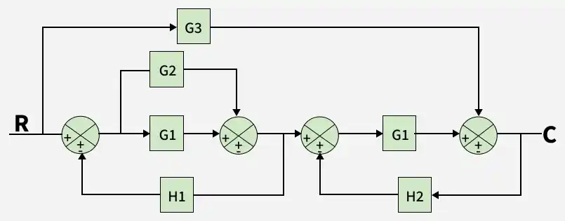
Figure 1

**Solution :

**Step 1 : G1 and G2 are connected in parallel , find its equivalent block G1 + G2

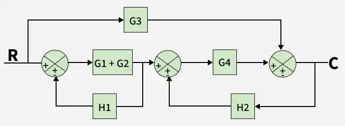
Figure 2

**Step 2 : Elimination of summing point before G1 + G2 having negative feedback H1 in closed loop system.

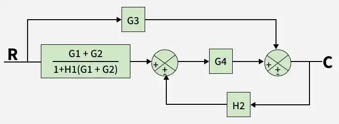
Figure 3

**Step 3 : Move summing point after G4 to before G4.

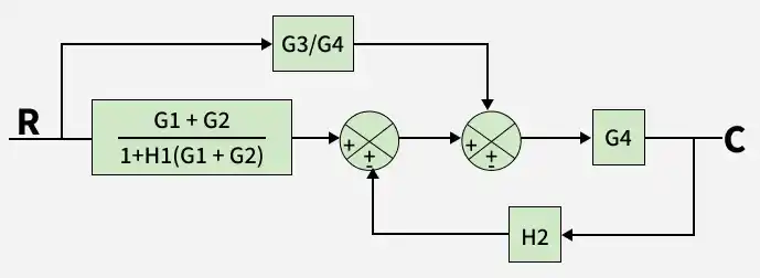
Figure 4

**Step 4 : Exchange the position of both the summing point before G4

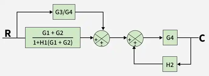
Figure 5

**Step 5 : G3 /G4 and (G1 +G2) / (1+G1H1+G2H2) both blocks are connected in parallel . Find equivalent block.

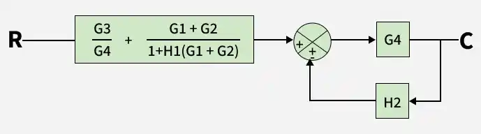
Figure 6

**Step 6 : Eliminate summing point before G4 having negative feedback in closed loop system.

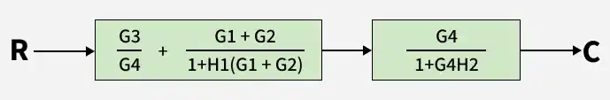
Figure 7

**Step 7 : Find the equivalent of both the cascaded block .

Single block diagram representation as shown below.

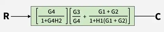
Figure 8