Mason's Gain Formula in Control System (original) (raw)
Last Updated : 9 Mar, 2026
Mason's Gain Formula, also known as Mason's Rule or the Signal Flow Graph Method, is a technique used in control systems and electrical engineering. It provides a systematic way to analyze the transfer function of a linear time-invariant (LTI) system, especially those with multiple feedback loops and complex interconnections.
- Mason’s Gain Formula (MGF) helps determine the transfer function of a linear signal flow graph.
- Total gain represents the relationship between input variables and output variables in a system.
- Signal labeling allows formation of equations that describe relationships among different signals.
- Solving those equations expresses the output signal in terms of the input signal.
**Mason's Gain Formula
Mason's gain formula for the determination of the overall system gain is given by:
T = \frac{C(s)}{R(s)} = \frac{\sum_{i=1}^{N}P_{i}\Delta_{i}}{\Delta}
where,
N: total number of forward paths
Pi : gain of the ith forward path
∆: determinant of the graph
∆i : path-factor for the ith path
The determinant of the graph (∆) and the path-factor for the ith path (∆i) are defined as follows:
∆i : 1 - (loop gain which does not touch the forward path)
∆: 1 - Σ(all individual loop gains) + Σ(gain product of all possible combinations of two non-touching loops) - Σ(gain product of all possible combinations of three non-touching loops) + ....
Important Terminologies of Mason's Gain Formula
- **Path: Traversal along connected branches where no node appears more than once.
- **Forward Path: Traversal from the input node to the output node.
- **Forward Path Gain: Product of all branch gains encountered along a forward path.
- **Loop: Closed path that begins and ends at the same node.
- **Non Touching Loops: Loops that do not share any common node.
- **Loop Gain: Product of branch gains along a closed loop.
Let us consider a signal flow graph for understanding the above elements:

Signal Flow Graph Showing Different Elements
**Forward Path
Form the above signal flow graph (SFG) image, there are two forward paths with their path gain as:
- P1 = ACEH
- P2 = AGH
**Loop
There are 4 individual loops in the above SFG with their loop gain as:
- L1 = BC
- L2 = EHD
- L3 = F
- L4 = GHDB
**Non-Touching Loops
There are ONE possible combinations of the non-touching loop with loop gain product as -
- L1.L3 = BCF
In above SFG, there are no combinations of three non-touching loops, 4 non-touching loops and so on.
Where,
- ∆1 = 1 (since all loops are touching P1)
- ∆2 = 1 (since all loops are touching p2)
- ∆ = 1- [L1+L2+L3+L4] + [L1.L3]
- ∆=1 - (BC + EHD + F + GHDB) + BCF
**Transfer Function:
\frac{C}{R}= \frac{P_{1}∆_{1}+P_{2}∆_{2}}{∆}
\frac{C}{R} = \frac{ACEH+AGH}{1-(BC+EHD+F+GHDB)+BCF}
Solved Examples on Mason Gain Formula
Example 1: Find the transfer function of the following signal flow graph
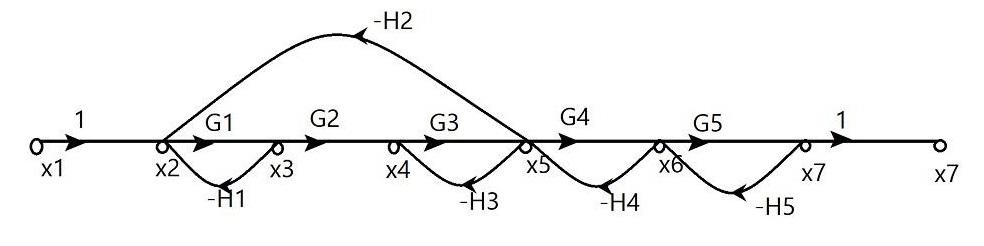
Signal Flow Graph
**Solution:
No. of forward path(N) = 1
Gain of Forward Paths (P1) = 1*G1G2G3G4G5
No. of individual loops:
- L1 = -G1H1
- L2 = -G3H3
- L3 = -G4H4
- L4 = -G5H5
- L5 = -G1G2G3H2
Non-Touching Loops (Combination of two):
- L1L2 = G1G3H1H3
- L1L3 = G1G4H1H4
- L1L4 = G1G5H1H5
- L24 = G3G5H3H5
- L4L5 = G1G2G3G5H2H5
Non-Touching Loops (Combination of three):
- L1L2L4 = -G1G3G5H1H3H5
Here,
**∆ 1 **= 1 (since all loops are touching p1)
**∆ = 1 - (L1+L2+L3+L4+L5) + (L1L2+L1L3+L1L4+L2L4+L4L5) - (L1L2L4)
**Transfer Function:
\frac{C}{R}=\frac{P_{1}∆_{1}}{∆}
\frac{C}{R} = \frac{G1G2G3G4G5}{(1+G1H1+G3H3+G4H4+G5H5+G1G2G3H2)+(G1G3H1H3+G1G4H1H4+G1G5H1H5+G3G5H3H5+G1G2G3G5H2H5)+(G1G3G5H1H3H5)}
Example 2: Find the transfer function of the following signal flow graph
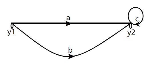
Signal Flow Graph
**Solution:
There are two forward paths and one loop. So, we have
- P1 = a
- P2 = b
- L1 = c
- ∆1 = ∆2 = 1 (since all loops are touching P1 & P2)
- ∆ = 1 - c
**Transfer Function:
\frac{C(s)}{R(s)}= \frac{a + b}{1 -c}
Example 3: Find the transfer function of the following signal flow graph
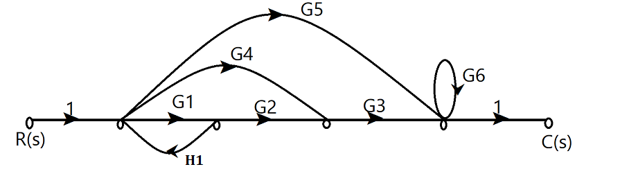
Signal Flow Graph
No. of forward path(N) = 3
The gain of Forward Paths:
- P1 = G1G2G3
- P2 = G4G3
- P3 = G5
No. of individual loops:
- L1 = G1H1
- L2 = G6
Non-Touching Loops (Combination of two)
- L1L2 = G1G6H1
∆1 = ∆2 = ∆3 = 1 (since all loops are touching P1,P2 &P3)
∆ = 1 - (G1H1+G6) + G1G6H1
**Transfer Function:
\frac{C(s)}{R(s)}= \frac{G1G2G3 +G3G4 + G5}{1-G1H1-G6 + G1G6H1}
Advantages & Disadvantages
**Advantages
- **Simplicity: A systematic procedure helps in calculating overall gain of a complex control system.
- **Comprehensive: Analysis remains possible even when several feedback loops exist in a system.
- **Versatility: Usage remains suitable for linear time-invariant control systems.
- **Visualization: Identification of different paths and loops becomes easier, which improves understanding of system behaviour.
Disadvantages
- **Complexity for Large Systems: Large numbers of loops and paths increase calculation difficulty and time.
- ****Limited to Linear Systems:**Application mainly focuses on linear time-invariant systems and does not directly support nonlinear or time-varying systems.
- **Assumption of Non Touching Loops: Analysis assumes loops do not intersect, which may not match some practical systems.
- **Limited Practical Insight: Calculation focuses on overall gain and may not clearly explain stability or dynamic characteristics required in some applications.
Applications
- **Stability Analysis: Calculation of poles and zeros of the overall transfer function helps in studying system stability.
- **Closed-Loop Systems: Evaluation of feedback effects helps in understanding overall system performance.
- **Transient and Steady-State Response: Study of system behaviour for transient conditions and steady-state inputs becomes easier.
- **Filter Design: Analysis of frequency response supports the design and development of filters.