Excel SUMIF Function: Formula and Examples (original) (raw)
Last Updated : 11 Mar, 2026
The SUMIF function in Excel adds values from a range that meet a specific condition. It helps you quickly calculate totals based on criteria like text, numbers, or dates, such as summing sales for a category or values within a certain date. This makes data analysis faster and easier.
**The simplest form of SUMIF Formula is:
SUMIF(range, criteria, [sum_range])
- **range: The range of cells you want to evaluate based on the criteria.
- **criteria: The condition that determines which cells to sum.
- **sum_range(optional argument): returns the sum of the sum_range or the range according to the given arguments
**Note: sum_range (optional): The range of cells to sum if different from the range to evaluate. If sum range not mentioned, it calculates the sum of same range as criteria condition.
**Return Value:
This function sums the numbers in the given range and returns the numerical value of the sum.
SUMIF Function in Excel
The SUMIF function is a useful tool, but it only takes a few simple steps to use it effectively. Here are the following steps to effectively use SUMIF in Excel formula.
Step 1: Open MS Excel
Step 2: Select the Cell for the Result
Select the cell in which you want to display the result of the SUMIF Function.
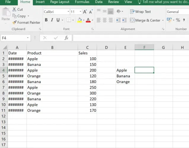
Select the cell to enter result
Step 3: Enter the SUMIF Function and specify the range
Start typing the Formula starting with the '=SUMIF' in the selected cell and also specify the range of the cells you want to evaluate. For example, if you want to evaluate cells 'B2' to 'B11', type 'B2:B11',.
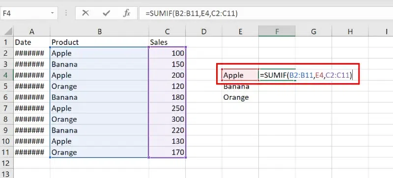
Type the Formula
Step 4: Define the Criteria
Enter the criteria for summing the values. For example, if you want to sum cells where the value is "Apple", Select cell E4(Apple).
Step 5: Drag the Formula
Step 6: Preview the Result
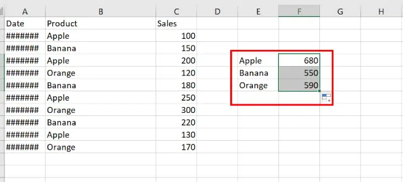
Preview the Result
Excel SUMIF with Dates
The SUMIF function with dates allows you to add values based on specific date criteria, ideal for tracking sales or events within a certain timeframe. For example, to sum all values after January 1, 2023, enter =SUMIF(B2:B11, ">01/01/2023", C2:C11).
Step 1: Open MS Excel
Step 2: Select the Cell
Select the cell in which you want to display the output.
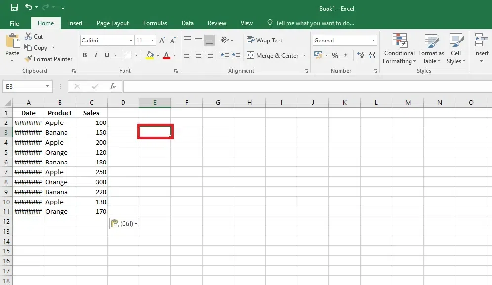
Select a Cell
Step 3: Enter the SUMIF Function and specify the range
Start by typing =SUMIF( in the selected cell and enter the range of cells the dates you want to evaluate. For example, if your dates are in column B from B2to B10, type B2:B10,.

Enter SUMIF function and specify range
Step 4: Define the Criteria
Enter the date criteria. For instance, if you want to sum values for dates after January 1, 2023, type " >01/01/2023",.

Define the Criteria
Step 5: Enter the Sum Range
Enter the range of cells that contain the values you want to sum. For example, if these values are in column B from B2 to B10, type B2:B10).

Enter the SUM Range
Example of SUMIF Function
An Excel sheet has been taken as an example and the SUMIF function has been used in several formats.
**Input:
| Coding Team names(Column A) | No. of members(Column B) | points(Column C) |
|---|---|---|
| GFG_CODERS | 4 | 200 |
| Acex_coders | 5 | 197 |
| Poisionous_python | 3 | 150 |
| Megatron | 4 | 130 |
| Bro_coders | 6 | 110 |
| Kotlin_coders | 2 | 100 |
| Gaming_coders | 3 | 50 |
Then we will apply the SUMIF() function to the above table:
| SUMIF() function | What the function does | Output result |
|---|---|---|
| =SUMIF(B2:B8, ">4", C2:C8) | If the no. of members in column B is greater than 4 then add the corresponding points of column C. | 307 |
| =SUMIF(B2:B8, 4, C2:C8) | If the no. of members in column B is equal to 4 then add the corresponding points of column C. | 330 |
| =SUMIF(A2:A8, "GFG_CODERS", C2:C8) | Search for "GFG_CODERS" in column A and add the corresponding points in column C. | 200 |
| =SUMIF(C2:C8, ">110") | Here the **sum_range argument is not provided. So it will check the cells of C column and if the points are greater than 110 add it to the result. | 677 |
| =SUMIF(A2:A8, "*rs", C2:C8) | Here it will find the names of the teams ending with "rs" / "RS" in column A and add the corresponding points to the sum. | 657 |
**Output:
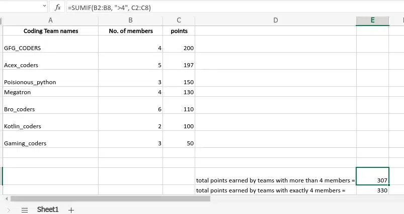
After Using the SUMIF Formula
SUMIFS with Multiple Criteria in Spreadsheet
Below are some examples of SUMIF Function in Excel:
Step 1: Enter the data Set
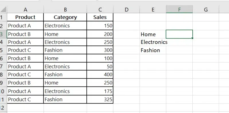
Enter the Data Set
Step 2: Enter the Formula for multiple criteria
=SUMIFS(sum_range, criteria_range1, criteria1, [criteria_range2, criteria2], ...)
- **sum_range: The range to add.
- **criteria_range1, criteria1: The first range and condition pair.
- **[criteria_range2, criteria2] (optional): Additional ranges and conditions.
Example: To sum the Sales where Product is "Product A" and Category is "Electronics":
=SUMIFS(C2:C10, A2:A10, "Product A", B2:B10, "Electronics")
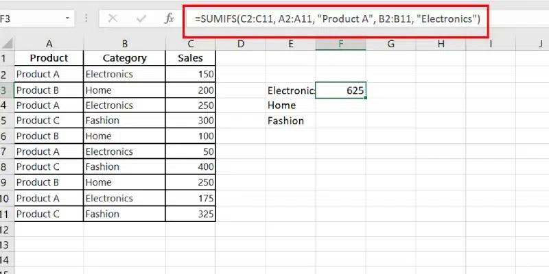
Enter the Formula