Excel: Modifying Columns, Rows, and Cells (original) (raw)
Last Updated : 23 Jul, 2025
Excel: Modifying Columns, Rows, and Cells - Quick Steps
- Open MS Excel
- Select Row, Column or a Cell
- Perform a Right-click >>Perform Actions
- Start Modifying
Excel is a powerful tool for organizing and managing data, and understanding how to efficiently modify rows, columns, and cells is crucial for anyone using it. Whether you're working with a **small spreadsheet or a **large dataset, being able to **change column widths, row heights, insert new rows or **columns, and **merge or unmerge cells will help you navigate Excel more effectively.
In this guide, we'll walk you through practical steps for modifying rows, columns, and cells, from **adjusting the size of rows and **columns to hiding or un-hiding them. We’ll also cover **how to wrap text and **merge cells, which are essential for better presentation and data organization in your spreadsheets.
**Disclaimer: Always save your work before making modifications to avoid accidental data loss.

Table of Content
- Row and Column in Excel
- How to Change Column Width in Excel (2 Methods)
- How to Change Row Height in Excel (2 Methods)
- Inserting, Deleting, Moving, and Hiding Rows and Columns
- Wrapping Text and Merging Cells
Row and Column in Excel
Before going further you should know what is a row in Excel and what is a column in Excel. You can see rows from left to right in an Excel file. Rows are groups of **horizontal rows. The maximum number of rows is **1,048,576. It goes across the **worksheet from left to right, following the data.
Excel columns may be easily distinguished by their alphabetical arrangement at the top of the spreadsheet. In addition, it goes from A to XFD. Excel has **16,384 columns, and the first one starts in Column A. Looking at the data from above in the spreadsheet, you'll see it flows vertically.
Working with Columns, Rows, and Cells
Working with columns, rows, and cells in Google Sheets allows you to organize and manipulate your data effectively. You can insert, delete, resize, or move rows and columns, as well as format individual cells to display data the way you need.
Whether you're adding new data, adjusting layout, or applying formulas, understanding how to manage these elements is key for efficient spreadsheet management.
How to Change Column Width in Excel (2 Methods)
Changing column width in Excel is essential for better organizing and displaying data. You may need to adjust column width to ensure your content fits neatly without being cut off or overlapping. There are two primary methods for adjusting column width: using the mouse to drag the column boundary or setting an exact width through the "Format" menu. Both methods allow for easy customization to enhance readability and presentation.
**Method 1: Double-Clicking the Column Border (Quick AutoFit)
If you want to quickly apply **AutoFit to a single column or multiple columns, you can use a **shortcut method by double-clicking the column border.
**Step 1: Select the Column Border
**Select the Column for which you want to **Change the Column Width.

Select the Column Border
Step 2: Place your Cursor between Column Headers until Double Arrow Cursor Appears
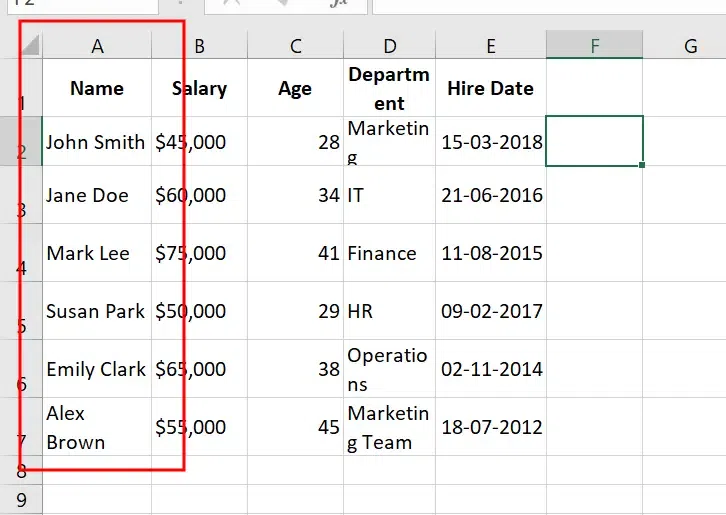
Position the cursor at the **right edge of the column header. Until it comes to double arrow icon. In the below example we want to Resize the Column A.

Place your Cursor between Column Headers >> Double Arrow Cursor Appears
**Step 2: Double-Click the Border
**Double-click the border between column headers. **Excel will automatically resize the column to fit the content.
Double Click the Border
**Alternate Method
You can also adjust the column width manually using the mouse. When the cursor turns into a double arrow, it indicates that resizing is possible. Simply click and drag the border left or right to adjust the width, then release the mouse button to finalize the change.
Method 2: Using AutoFit Column Width Feature
AutoFit automatically **adjusts the column width to fit the **largest content in that column. This method is very useful when you have varying **text or **data lengths and need the column to expand or contract accordingly. Follow the below **steps to use AutoFit Column Width:
Step 1: Select the Column(s)
**Click on the column letter(s) to select the columns you want to resize. In the below example we have selected **Column A,B,C and D.
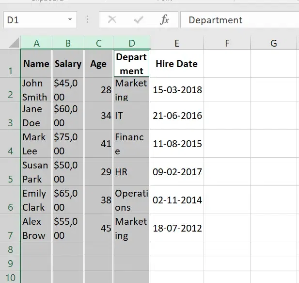
Select the Columns
Step 2: Go to the Home Tab and Select Format
On the **Excel Ribbon, navigate to the Home tab and In the "**Cells" section of the Ribbon, **find and click Format.

Home Tab>>Click on Format
Step 3: Select AutoFit Column Width
From the **drop-down menu, click AutoFit Column Width. Excel will automatically adjust the column width to **match the largest content in that column.
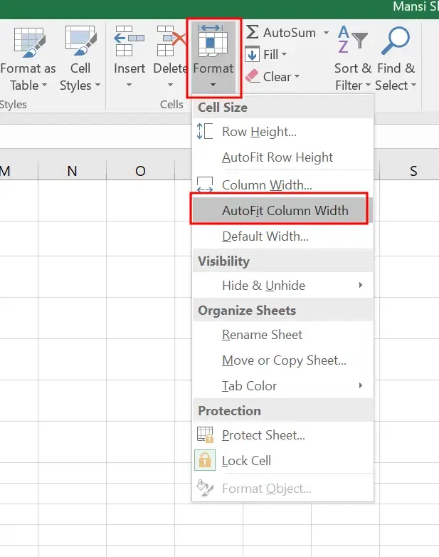
Select Autofit Column Width
**Alternative Method
You can also manually set the column width by clicking on "**Column Width" and **enter the column width size.
**Shortcut to Set Column Width:
**Windows: Press **Alt + H + O + W to manually input column width.
**Mac: Press **Control + Option + W to set the width manually.
Step 4: Preview Result
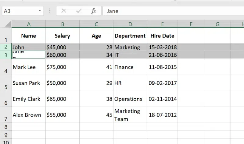
In the following result, the **column widths are adjusted to fit the largest content within each column.

Columns are Resized
How to Change Row Height in Excel (2 Methods)
Changing row height in Excel helps improve data visibility and organization, especially when text or content doesn't fit properly within the cells. There are two simple methods for adjusting row height: using the **Double Click Method, where you double-click the row boundary to auto-adjust to the content, or using the **Ribbon (AutoFit) option, which automatically resizes the row to fit the largest content in the cells.
Both methods allow you to customize the layout and make your spreadsheet more readable.
Method 1: Using Double Click Method
This method allows you to quickly change your row height in excel to fit your text in excel. Follow the below steps to change row height in Excel:
Step 1: Select the Row(s)
**Click on the row number of the row you want to adjust. You can select a **single row or **multiple rows. Here we have selected Row 2 and **Row 3.
Select the Rows
Step 2: Hover Over the Row Border and Double-Click the Border
Move your cursor to the bottom edge of the selected row number (**the horizontal line between two row numbers). When you hover over this border, the cursor will change to a double-headed arrow. Once the **double-headed arrow appears, **double-click on the row border.
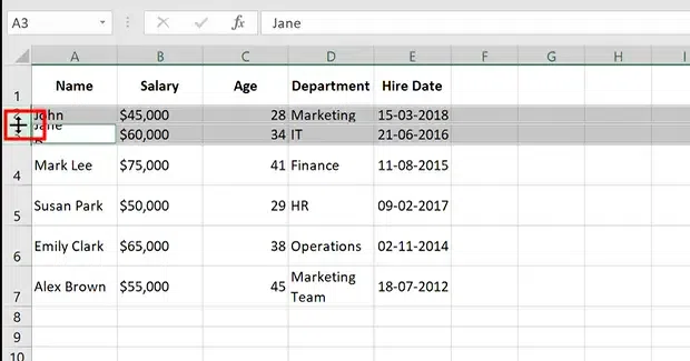
Double Click the Row Border
Step 3: Preview Result
Excel will automatically **adjust the row height to fit the largest content in that row. The row will **expand or **shrink depending on the content's height.

Preview Results
**Alternate Method
You can also adjust the row height manually by clicking and holding the mouse button on the row border, then dragging it upwards to reduce the height or downwards to increase it.
Method 2: Using the Ribbon (AutoFit)
If you want to automatically adjust the **row height to fit the largest content in the row, you can use AutoFit.
Step 1: Select the Row(s)
Click on the **row number(s) to **select the row(s) you want to modify.
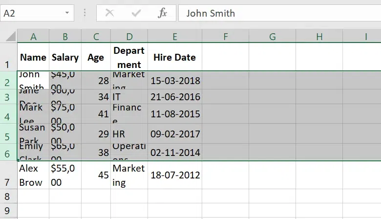
Select the Rows
Step 2: Go to the Home Tab and Click on Format
On the Excel ribbon, go to the Home tab and Select Format option in the Cells Group.
Step 3: Select AutoFit Row Height
From the dropdown, choose AutoFit Row Height. The row height will automatically adjust to fit the tallest content.
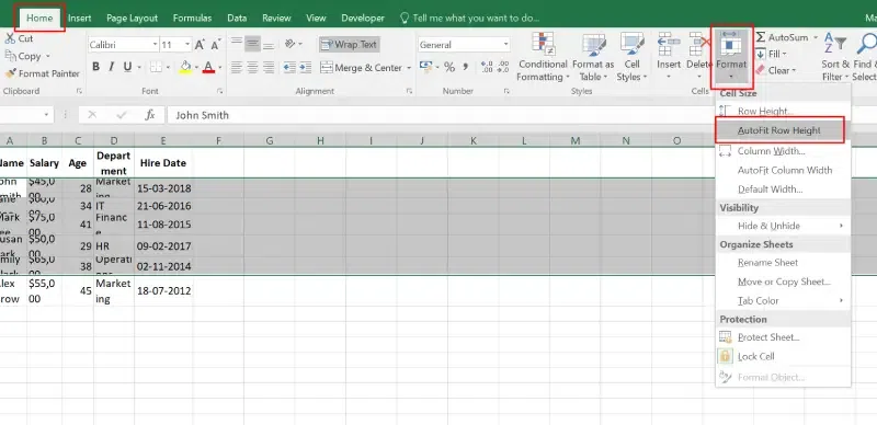
Select the Rows >> Go to Home Tab>> Click on Format Option and Select Autofit Row Height
**Alternate Method
You can select "Row height" to manually to set a specific row height by entering a value.
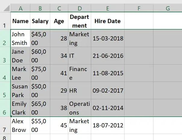
Step 4: Preview Results
In the below result, all the columns are set to the Autofit Row Height in Excel.
Preview Results
Inserting, Deleting, Moving, and Hiding Rows and Columns
In Excel, managing rows and columns is essential for organizing data efficiently. You can **insert, **delete, **move, or **hide rows and columns as needed to better structure your worksheet. **Inserting rows or columns adds new space for data, while **deleting removes unnecessary ones.
**Moving rows or columns allows you to rearrange data, and **hiding rows or columns helps to temporarily conceal irrelevant information without removing it. These actions can be done easily through the **right-click menu or ribbon options, making it simple to adjust the layout of your spreadsheet.
How to Insert a Row in Excel (3 Methods)
In Excel, you can insert a row using three methods: the **keyboard shortcut for a fast insertion, the **right-click menu by selecting a row and choosing "**Insert," or the **ribbon (Home tab) by clicking the "**Insert" option. Each method provides a quick way to add a new row based on your preference.
Method 1: Using Keyboard Shortcuts (Fast Method)
To **Insert a Row quickly this method is best for you:
Step 1: Select the Row
**Click on the row number where you want the new row to appear. Here, we want to **insert a new row above row 3, so we have **selected row 3.

Select the Row
Step 2: Press Ctrl + Shift + "+" and Preview Result
**Press Ctrl + Shift + "+" on your keyboard for windows and Press Command + Shift + "+" for mac. A new row will be inserted above the selected row.

Row has been Inserted
This is one of the quickest ways to insert a row when working with Excel.
Step 1: Select the Row
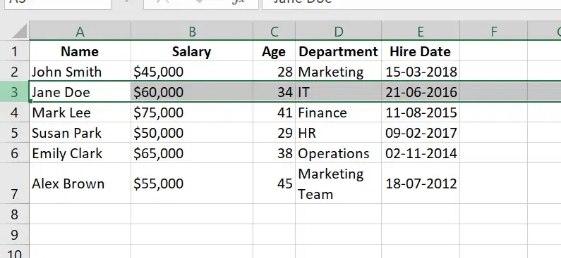
Click on the row number where you want the new row to appear. The row will be inserted above the selected row. Here we have selected row 5.
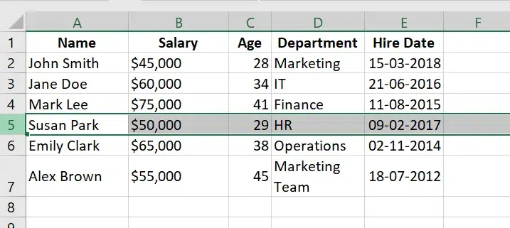
Select the Row
Step 2: Right-Click and Choose Insert
Right-click on the selected row number. From the context menu that appears, click Insert. A new row will be inserted above the selected row.
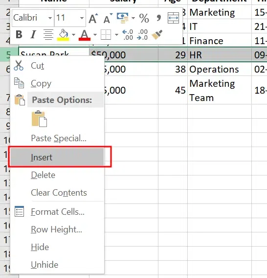
Right Click and Choose Insert
Step 3: Preview Result
New row has been inserted now.
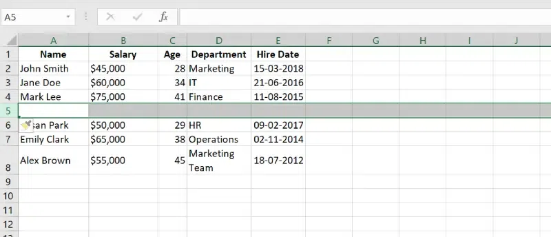
Preview Results
Method 3: Using the Ribbon (Home Tab)
If you prefer using the Excel Ribbon, you can insert a row directly through the Home tab.
Step 1: Select the Row
Click on the row number where you want the new row to appear. In the below example we have selected Row 7.
Step 2: Go to Home Tab ,Click on Insert option and Select Insert Sheet Rows
On the top menu, go to the Home tab. In the Cells group, click Insert, then select Insert Sheet Rows.

Select the Row>> Go to Home tab>> Click on Insert Tab
Step 3: Preview Results
A new row will be inserted above the selected row.
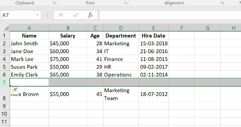
New Row has been Inserted
How to Insert Columns in Excel (3 Methods)
To insert columns in Excel, you can use three methods: **keyboard shortcuts for a quick insertion, the **right-click method by selecting a column and choosing "Insert," or the **ribbon (Insert command) by selecting the "Insert" option under the Home tab. These methods allow for efficient column insertion based on your preferred workflow.
Method 1: Using Keyboard Shortcuts
To **Quickly Insert columns in Excel you can use **Keyboard shortcuts, Follow the below steps to insert columns in Excel:
Step 1: Select the Column
**Click on the column heading where you want to **insert the new column. Here we have selected Column B.
Select the Column
Step 2: Use the Shortcut ( Press Ctrl + Shift + "+" )
Press **Ctrl + Shift + "+" (plus sign) for windows and **Press Command + Shift + "+" for mac on your keyboard to instantly insert a new column to the left of the selected column.
Step 3: Preview Results
Now you can see that the new blank column has been inserted to left of selected column.

Preview Results
Method 2: Right-Click Method
Follow the below steps to Insert a new blank column in excel, using right click method:
Step 1: Select the Column
Click on the column heading to the right of where you want the new column. Here we have selected Column D.
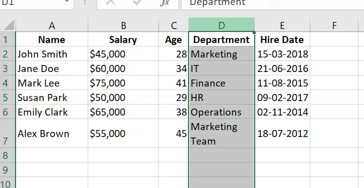
select the Column
Step 2: Right-Click on the Column and Select "Insert"
Right-click on the selected column heading. From the context menu that appears, select Insert. A new column will be inserted to the left of the selected column.
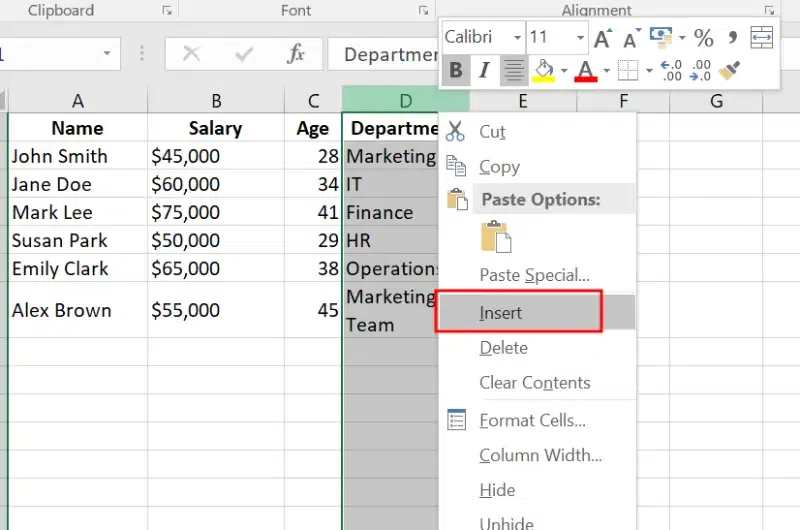
Right click and Select Insert
Step 3: Preview Results
New column has been inserted.
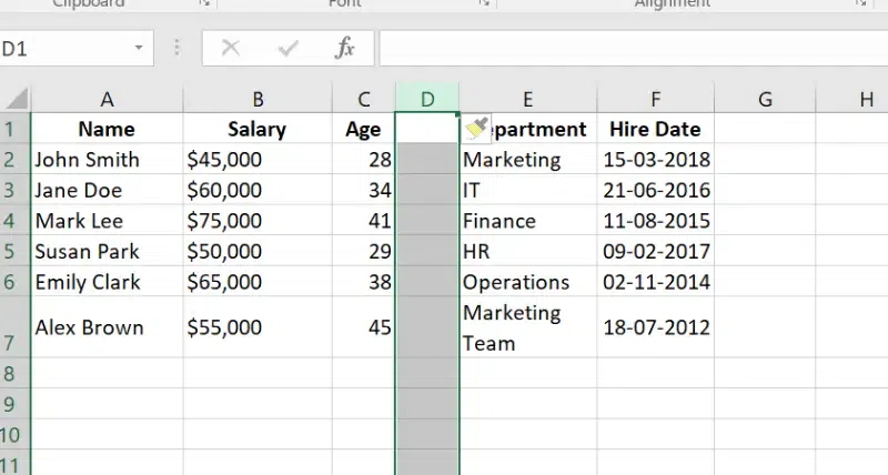
New Column has been inserted
Method 3: Using the Ribbon (Insert Command)
To insert a column **using the Ribbon in Excel, follow these steps:
Step 1: Select the Column(s)
Click on the column heading (**e.g., "B", "C", etc.) to the right of where you want the new column to be inserted. To select multiple columns, **hold down the Shift key and **click on the column numbers.
Step 2: Go to the "Home" Tab, Click the "Insert" Command and Select Insert Sheet Columns
Navigate to the Home tab on the Excel ribbon. In the Cells group, click on the Insert dropdown, and then select Insert Sheet Columns. This will insert a new column to the left of the selected column.
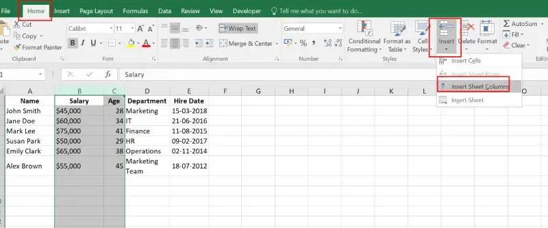
Home tab>> Click on Insert>> Select Insert Sheet Columns
Step 3: Preview Results
**New columns has been Inserted.
New columns has been Inserted
How to Delete a Column or Row (3 Methods)
To delete a column or row in Excel, you can use three methods: **keyboard shortcuts for fast removal, the **right-click menu by selecting the column or row and choosing "Delete," or the **ribbon by clicking on "**Delete" in the Home tab. Each method provides a quick and easy way to remove unwanted rows or columns.
Method 1: Using Keyboard Shortcuts
This is the fastest way to delete a Column or Row in excel:
Step 1: Select the Column or Row
Click the column or row header to select it. Here we want to remove column A.
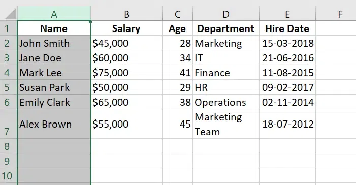
Select the Column or Row to Delete
Step 2: Press the Delete Shortcut and Preview Result
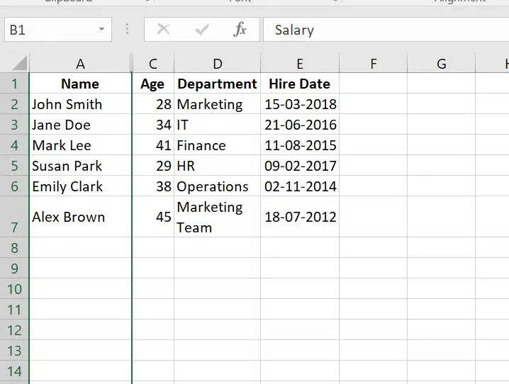
Use the keyboard shortcut Ctrl + "-" (minus) for windows and Press Command + "-" (minus) for mac to delete the selected row or column. This will remove the Column. Column "**Salary" has been removed.

Column A "Salary" has been removed
You can use the **Right click menu to Remove a column or row in Excel worksheet. Follow the below steps to delete a row or column in Excel:
Step 1: Select the Column or Row
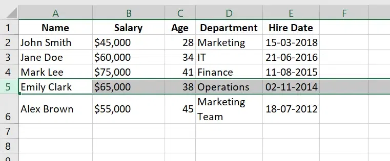
Click on the **column or row header (the letter for columns or number for rows) to select it. Here we have selected **Row 5.
Step 2: Right-Click and Choose Delete
**Right-click the selected column or row header. From the context menu, click **Delete.
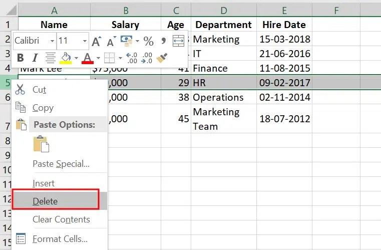
Right Click and Select Delete
Step 3: Preview Result
**Selected row or **column has been removed from your worksheet.
Preview Result
Method 3: Using the Ribbon
You can use this method to remove the column or row from the Excel Worksheet:
Step 1: Select the Column or Row
Click on the column or row header that you want to delete.
Step 2: Go to the Home Tab and Select Delete
On the **Excel ribbon, go to the **Home tab, In the **Cells group, **click on the Delete button to remove the selected row or column.
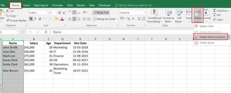
Select Column or Row >> Choose Delete>> Select Delete Sheet Columns
These methods will remove the **row or **column entirely from your worksheet. Be mindful, as this action cannot be undone once completed, unless you immediately use **Ctrl + Z to undo the deletion.
How to Move a Row or Column
Moving rows or columns in Excel is a useful technique when you want to rearrange data without deleting and re-entering it. There are several methods to move rows or columns in Excel.
Method 1: Using Right Click Method
To Quickly Move a Column or Row in Excel, use can use the Right Click method:
Step 1: Select the Row or Column
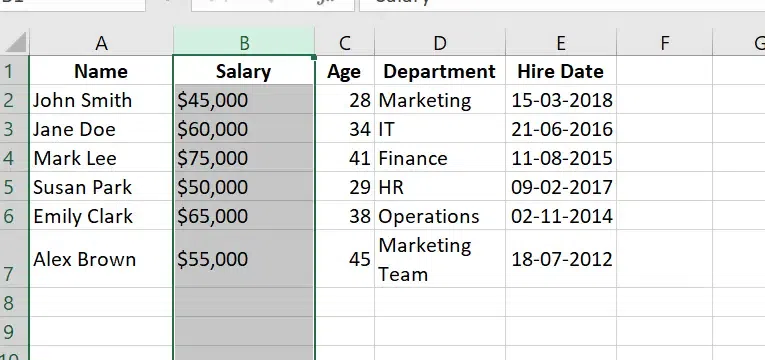
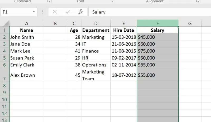
Click the row number or column letter to select the row or column you want to move. Here we have selected Column B (Salary).
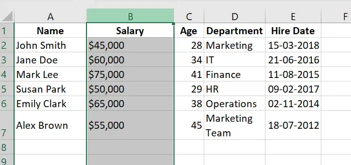
Select the Row or Column
Step 2: Right Click and Select Cut the Row or Column
**Right click and **select the Cut Option or Press **Ctrl + X to cut the row or column.
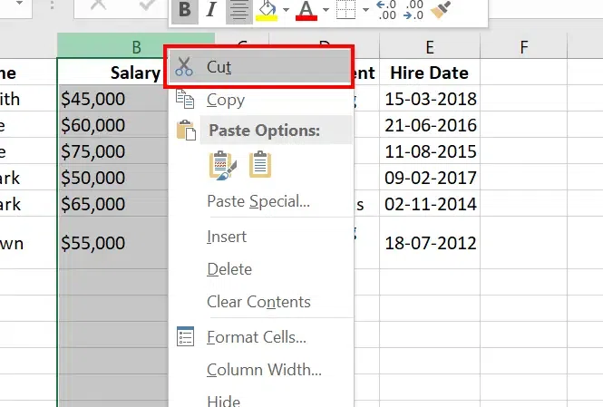
Right Click >> Select the "Cut" Option
Step 3: Select the New Location
**Click the row number or column letter where you want to move the data. Here, we have **selected Column F.
- If moving a row, position the cursor over the row number.
- If moving a column, position the cursor over the column letter.
Step 4: Right Click Paste the Cut Row/Column
**Right Click and **Select Paste or Press Ctrl + V to **paste the cut row or **column in the new location. (**Here Column F).

Right Click and Select Paste Option
Step 5: Preview Results
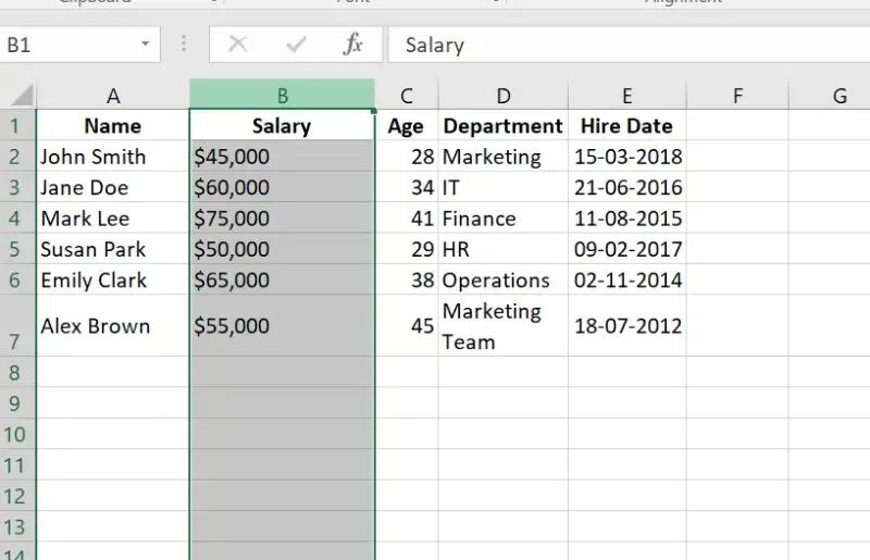
Salary has been moved to **new column F.
Salary has been shifted.
**Note:
- When you move a column or row, the data, formatting, and formulas associated with that row or column are also moved.
- You cannot move a row or column to a location that already contains data without overwriting it. Be sure the destination area is empty or prepared for the change.
You may want to compare specific rows or columns without rearranging your worksheet every time. You can hide rows and columns in Excel as needed to do this.
How to Hide Rows or Columns in Excel (2 Methods)
There are different methods to Hide Columns and Rows.
Method 1: Using Shortcuts
This is the quick way to hide a row or column using shortcuts:
Step 1: Select the Row or Column
Click the row number or column letter to select it. Here we have selected the Column B.
Column B Selected
Step 2: Use the Shortcut
**Press Ctrl + 9 to hide a row, or Ctrl + 0 to hide a column in windows and for mac **Press Command + Shift + 9 to unhide rows.
**Press Command + Shift + 0 to unhide columns.
Step 3: Preview Result
**Selected row is Hidden now.
Preview Results
This is the easiest way to Hide Row or Column in Excel:
Step 1: Select the Row or Column
Click the **row number or **column letter of the row or column you want to hide. Here we have Selected Row "3".
Select the Row or Column you want to hide
Step 2: Right-click and Select Hide
Right-click on the selected row or column. From the context menu, select **Hide.
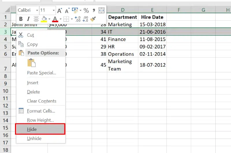
Right Click and Select Hide
Step 3: Preview Result
The row or column will disappear from view.
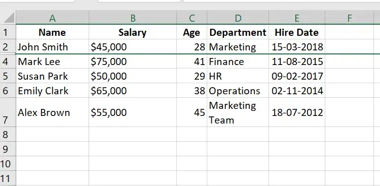
Preview Result
How to Unhide a Row or Column in Excel
If you’ve hidden rows or columns in Excel, you can easily unhide them using several methods. Here’s how to unhide rows or columns step by step:
Method 1: Using Keyboard Shortcuts
To quickly unhide a row or column in Excel, you can use keyboard shortcuts. This method is fast and efficient for uncovering hidden data without needing to use menus.
Step 1: Select Adjacent Rows or Columns
**Highlight the rows or **columns next to the hidden row or **column. Here **Row 5 is hidden, so we have selected **Row 4 and Row 6.
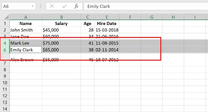
Adjacent Rows Selected.
Step 2: Use the Shortcut and Preview Results
**Press Ctrl + Shift + 9 to unhide rows for windows and Press Command + Shift + 9 to unhide rows in mac.
**Press Ctrl + Shift + 0 to unhide columns (may require enabling in system settings).
This will unhide the hidden column or Rows:
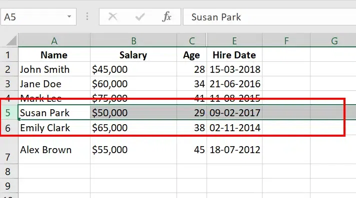
Preview Results
Method 2: Using the Ribbon
To unhide a row or column using the Ribbon, follow these steps:
Step 1: Select Adjacent Rows or Columns
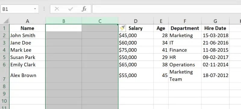
**Highlight the rows or **columns surrounding the hidden area. Here **Column B is hidden so we have selected Column A and **Column C.
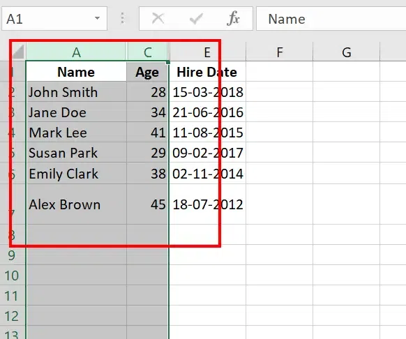
Select the Adjacent Columns
Step 2: Go to the Home Tab, Click on Format Drop Down, Select Hide Unhide and Choose your Option
On the Excel ribbon, click the Home tab, In the Cells group, click the Format dropdown menu Select Hide & Unhide, and from the submenu, select either Unhide Rows or Unhide Columns.
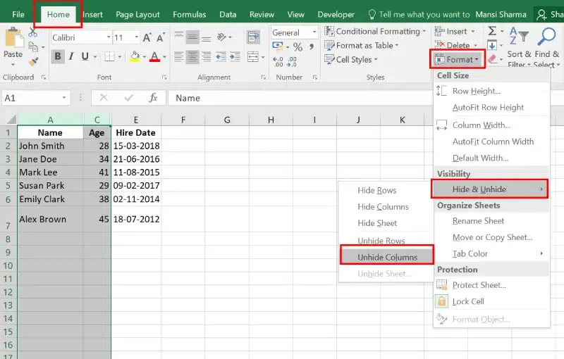
Go to Home Tab >>Format>>Hide and Unhide>> Unhide Columns
**Alternate Method:
After selecting the Adjacent Rows or Columns, Right and Select Unhide. This is will unhide the hidden rows or column.
Step 3: Preview Results
The hidden row or column will become visible.
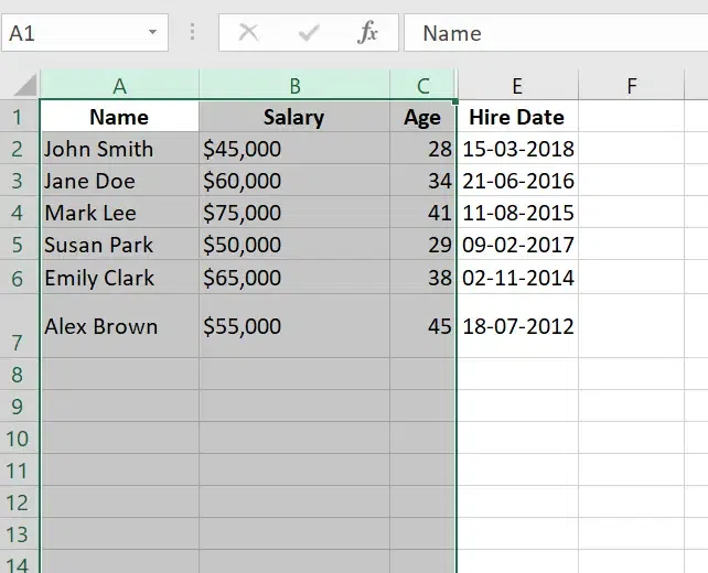
Preview Results
Wrapping Text and Merging Cells
Wrapping text in Excel allows you to display all the text within a cell by adjusting its height to fit multiple lines. This ensures that the content remains visible without overflowing into adjacent cells.
How to Wrap Text in Excel
Learn how to wrap text in Excel cells to keep your data neat and readable. Follow easy steps to ensure text fits within the cell without overflowing, improving the layout and organization of your spreadsheet.
Method 1: Using Keyboard Shortcut
To wrap text in Excel quickly, you can use a keyboard shortcut. This will make the text in the selected cell automatically wrap within the cell, adjusting the row height if necessary.
Step 1: Select the Cells
**Select the cells in which you want to text Wrap.
Select the Cells
Step 2: Press Alt + H +W Shortcut and Preview Results
Press Alt + H first and then press W for windows and **Press Command + Option + W to wrap text in the selected cell(s) and Preview Results.

Press Alt +H+W and Preview Results.
Method 2: Using the Ribbon
The **Ribbon method in Excel is an easy way to wrap text within a cell to make sure it fits neatly without overflowing. By using the Ribbon, you can quickly apply text wrapping without manually adjusting row height or column width.
Step 1: Select the Cell(s)
Click on the **cell or **range of cells where you want to wrap text.

Select the Cells
Step 2: Go to the Home Tab and Select Wrap Text
On the Ribbon, navigate to the Home tab and In the **Alignment group, **click the Wrap Text button. The text in the **selected cell(s) will automatically adjust to fit within the column width, creating multiple lines if necessary.
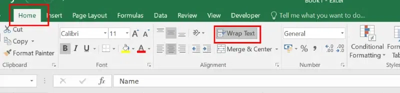
Home tab>> Wrap Text
Step 3: Preview Results
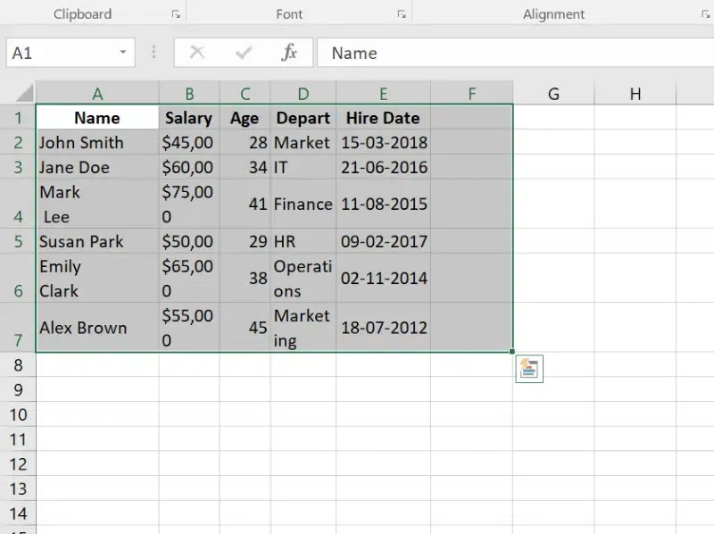
The text in the selected cell(s) will automatically **adjust to fit within the column width, creating multiple lines if necessary.

Preview Results
How to Merge Cells in Excel
Merging cells in Excel is a common formatting task used to combine multiple adjacent cells into a single, larger cell. This is often done for **better alignment, **creating headers, or improving the visual layout of a spreadsheet. Here are the different methods to merge cells in Excel:
Method 1: Using Keyboard Shortcuts
The **keyboard shortcut method is the quickest way to merge cells in Excel. It’s especially helpful for users who are comfortable with keyboard shortcuts and want to speed up their workflow.
Step 1: Select the Cells you want to merge
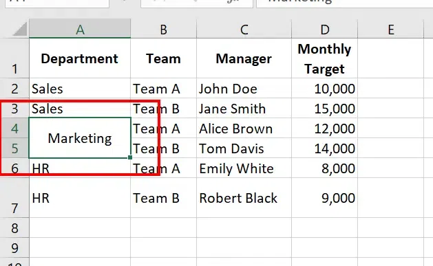
**Select the Cells you want to merge. Here we have selected **Sales (A2 and A3) to merge:
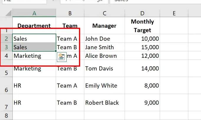
Select the cells to merge
Step 2: Press Alt +H + M +C Shortcuts to Merge and Preview Results
**Press Alt +H at first and then press M and **lastly C in windows and **Control + Command + M for Mac. This will merge and Centre your cells.
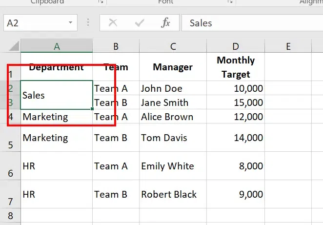
Use shortcuts Alt+H+M+C and Preview Merged Cells
Method 2: Using Ribbon (Merge & Center Feature)
The **Merge & Center feature in Excel allows you to **merge multiple cells into one larger cell and **center the content within it. Using the Ribbon for this process is quick and straightforward, as it provides a clear button to **merge and center cells with just a few clicks.
Step 1: Select the Cells
**Highlight the cells you want to merge.
Step 2: Go to the Home Tab and Select "Merge and Center"
Navigate to the **Home tab on the Excel Ribbon, In the Alignment group, **click the Merge & Center button.
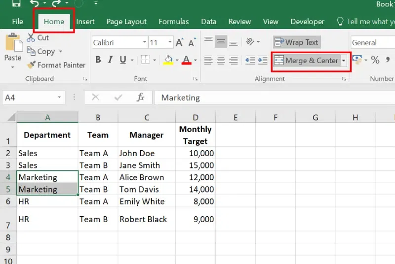
Select the cells>> Go to Home Tab>>Select Merge and Centre
Step 3: Preview Results
The **selected cells will be merged into one, and the text (if any) will be centered.
Preview Results
You can also choose other options, such as "**Merge Across" or "**Merge Cells," to merge without centering, depending on the requirements of your dataset.
To learn other methods of merge and unmerge cells click here.
Conclusion
Modifying columns, rows, and cells in Excel is more than just a formatting task—it's a way to make your spreadsheets work for you. By learning to change **column width and **row height, insert or delete rows and columns, and move rows or columns effortlessly, you can maintain a well-organized and visually appealing worksheet.
Advanced features like **wrapping text, merging cells, or hiding and unhiding rows or **columns ensure your data looks neat and professional. Whether you're handling a simple list or a complex dataset, mastering these Excel techniques will empower you to manage your data efficiently and impressively.