Pivot Tables in Excel (original) (raw)

Last Updated : 9 Jun, 2026

Pivot Tables in Excel are a useful tool for summarizing, analyzing and organizing large datasets. They allow users to group, filter, and perform calculations like sums and averages using a simple drag-and-drop interface.

Creating a Pivot Table in Excel

Follow these simple steps to build a Pivot Table in Excel:

Step 1: Preparing the Data

Before creating a Pivot Table, ensure our data is properly formatted:

• **Organize in a Tabular Format: Place our data in rows and columns, with each column having a header.
• **Avoid Blank Rows or Columns: Ensure there are no empty rows or columns within our dataset.
• **Name our Data Range (Optional): Highlight our data and assign a name with Formulas > Define Name for easier reference.

Prepare your Data

Step 2: Selecting the Data

1. Click any cell inside our data or
2. Highlight the specific range we want to include in the Pivot Table.

Step 3: Inserting a Pivot Table

• Go to the Insert tab on the Excel ribbon.
• Click PivotTable.
• In the Create PivotTable dialog box:
• Verify the selected data range.
• Choose the location:
• **New Worksheet: Places the Pivot Table in a new sheet (recommended).
• **Existing Worksheet: Specify a cell in the current sheet.

Select your Data >>Go to Insert Tab>> Select Pivot Table

**Shortcut Keys:

• **Windows: Press Alt + N + V to open the Create PivotTable dialog box.
• **Mac: Press Command + Option + P to create a Pivot Table.

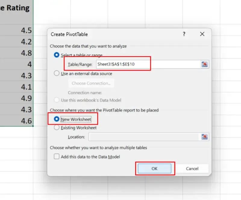
Select your Range>> Select your Sheet and Press OK

Step 4: Build our Pivot Table

We'll see a PivotTable Field List pane on the right side of our screen. This is where we organize our data:

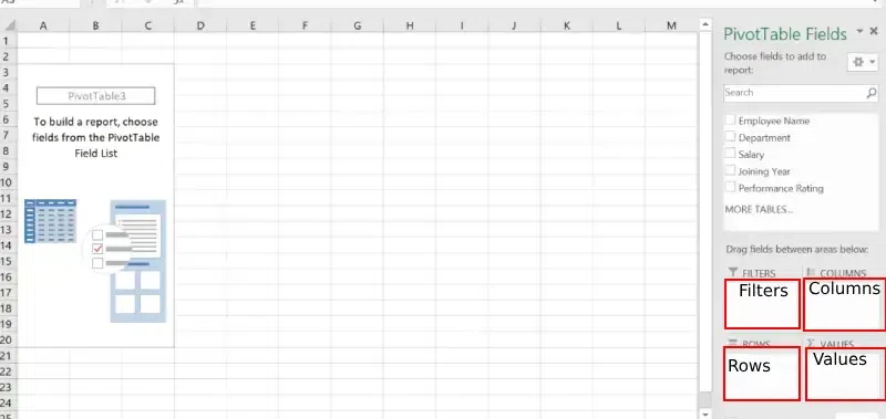
Build your Pivot Table

**a) Drag and Drop Fields:

Drag column headers from the Field List into one of the four areas:

• **Rows: Sets rows for the table.
• **Columns: Creates columns for our data.
• **Values: Adds numerical data to be calculated like sum, count, etc.
• **Filters: Adds filters to refine our analysis.

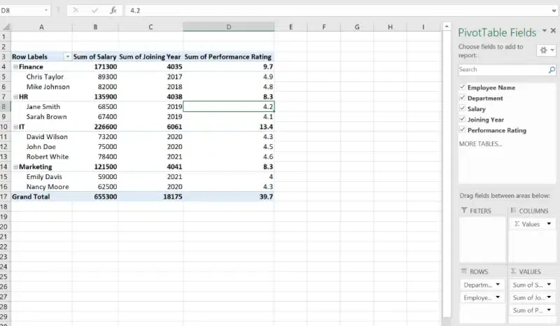
Drag the Fields

**b) Customize Calculations:

Right-click on a value in the Values area and choose Value Field Settings. Then, Select the desired calculation like Sum, Average, Count, etc.

Step 5: Formatting and Customizing the Pivot Table

• **Apply a PivotTable Style: Select the Pivot Table and go to Design > PivotTable Styles to apply a pre-designed format.
• **Sort and Filter: Use the dropdown arrows on row or column headers to sort and filter data.
• **Group Data: Right-click on a row or column item and select Group to organize data by date, number ranges etc.
• **Add Slicers (Optional): Go to Insert > Slicer to create interactive filters for our Pivot Table.

**Shortcut Key:

Windows: Press Alt → J → T → F (sequentially) to open the Field List pane; Mac: no default shortcut available use PivotTable Analyze → Field List.

Step 6: Refresh the Pivot Table

Update the Pivot Table when source data changes. Click anywhere in the Pivot Table.

• Going to PivotTable Analyze > Refresh.

**Select Entire Pivot Table Shortcut Key: For Windows/Mac, Press Ctrl + A (or Command + A on Mac) to select the entire Pivot Table.

Analyze >> Refresh