Gradient Descent in Linear Regression (original) (raw)

Last Updated : 27 May, 2025

**Gradient descent is a optimization algorithm used in **linear regression to find the best fit line to the data. It works by gradually by adjusting the line’s slope and intercept to reduce the difference between actual and predicted values. This process helps the model make accurate predictions by minimizing errors step by step. In this article we will see more about Gradient Descent and its core concepts in detail.

Linear-Regression

Gradient Descent in Linear Regression

Above image shows two graphs, left one plots house prices against size to show errors measured by the **cost function while right one shows how **gradient descent moves downhill on the cost curve to minimize error by updating parameters step by step.

Why Use Gradient Descent for Linear Regression?

Linear regression finds the **best-fit line for a dataset by minimizing the **error between the actual and predicted values. This error is measured using the cost function usually Mean Squared Error (MSE). The goal is to find the model parameters i.e. the **slope m and the **intercept b that minimize this cost function.

For simple linear regression, we can use formulas like Normal Equation to find parameters directly. However for **large datasets or **high-dimensional data these methods become computationally expensive due to:

Large matrix computations.
Memory limitations.

In models like polynomial regression, the cost function becomes highly complex and non-linear, so analytical solutions are not available. That’s where **gradient descent plays an important role even for:

Large datasets.
Complex, high-dimensional problems.

**How Does Gradient Descent Work in Linear Regression?

Lets see various steps involved in the working of Gradient Descent in Linear Regression:

**1. Initializing Parameters: Start with random initial values for the slope (m) and intercept (b).

**2. Calculate the Cost Function: Measure the error using the Mean Squared Error (MSE):

J(m, b) = \frac{1}{n} \sum_{i=1}^{n} \left( y_i - (mx_i + b) \right)^2

**3. Compute the Gradient: Calculate how much the cost function changes with respect to m and b.

For slope m :

\frac{\partial J}{\partial m} = -\frac{2}{n} \sum_{i=1}^{n} x_i (y_i - (mx_i + b))

For intercept b:

\frac{\partial J}{\partial b} = -\frac{2}{n} \sum_{i=1}^{n} (y_i - (mx_i + b))

**4. Update Parameters: Change m and b to reduce the error:

For slope m :

m = m - \alpha \cdot \frac{\partial J}{\partial m}

For intercept b :

b = b - \alpha \cdot \frac{\partial J}{\partial b}

Here \alpha is the learning rate that controls the size of each update.

**5. Repeat: Keep repeating steps 2–4 until the error stops decreasing significantly.

Implementation of Gradient Descent in Linear Regression

Let’s implement linear regression step by step. To understand how gradient descent improves the model, we will first build a simple linear regression without using gradient descent and observe its results.

Here we will be using Numpy, Pandas, Matplotlib and Sckit learn libraries for this.

**X, y = make_regression(n_samples=100, n_features=1, noise=15, random_state=42): Generating 100 data points with one feature and some noise for realism.
**X_b = np.c_[np.ones((m, 1)), X]: Addind a column of ones to X to account for the intercept term in the model.
**theta = np.array([[2.0], [3.0]]): Initializing model parameters (intercept and slope) with starting values. Python `

import numpy as np import matplotlib.pyplot as plt from sklearn.datasets import make_regression

X, y = make_regression(n_samples=100, n_features=1, noise=15, random_state=42) y = y.reshape(-1, 1) m = X.shape[0]

X_b = np.c_[np.ones((m, 1)), X]

theta = np.array([[2.0], [3.0]])

plt.figure(figsize=(10, 5)) plt.scatter(X, y, color="blue", label="Actual Data") plt.plot(X, X_b.dot(theta), color="green", label="Initial Line (No GD)") plt.xlabel("Feature") plt.ylabel("Target") plt.title("Linear Regression Without Gradient Descent") plt.legend() plt.show()

**Output:

download2

Linear Regression without Gradient Descent

Here the model’s predictions are not accurate and the line does not fit the data well. This happens because the initial parameters are not optimized which prevents the model from finding the best-fit line.

Now we will apply **gradient descent to improve the model and optimize these parameters.

**learning_rate = 0.1, n_iterations = 100: Set the learning rate and number of iterations for gradient descent to run respectively.
**gradients = (2 / m) * X_b.T.dot(y_pred - y): Finding gradients of the cost function with respect to parameters.
**theta -= learning_rate * gradients: Updating parameters by moving opposite to the gradient direction. Python `

learning_rate = 0.1 n_iterations = 100

for _ in range(n_iterations):

y_pred = X_b.dot(theta)

gradients = (2 / m) * X_b.T.dot(y_pred - y)

theta -= learning_rate * gradients

plt.figure(figsize=(10, 5)) plt.scatter(X, y, color="blue", label="Actual Data") plt.plot(X, X_b.dot(theta), color="red", label="Optimized Line (With GD)") plt.xlabel("Feature") plt.ylabel("Target") plt.title("Linear Regression With Gradient Descent") plt.legend() plt.show()

**Output:

download3

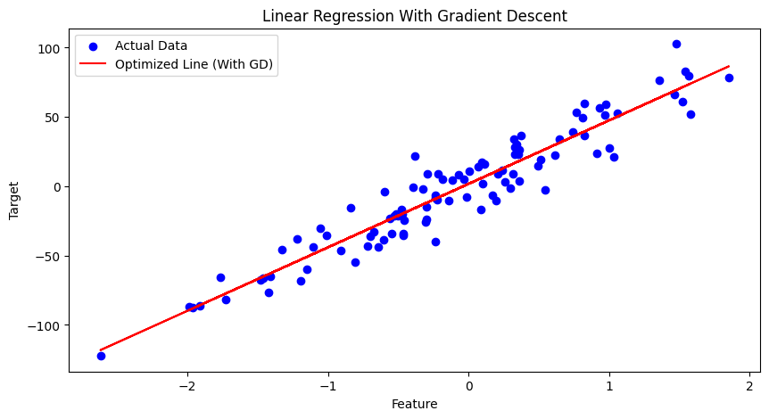
Linear Regression with Gradient Descent

Linear Regression with Gradient Descent shows how the model gradually learns to fit the line that minimizes the difference between predicted and actual values by updating parameters step by step.

As datasets grow larger and models become more complex, gradient descent will continue to help in building accurate and efficient machine learning systems.