Implementation of Lasso Regression From Scratch using Python (original) (raw)

Last Updated : 13 Apr, 2025

Lasso Regression (Least Absolute Shrinkage and Selection Operator) is a linear regression technique that combines prediction with feature selection. It does this by adding a penalty term to the cost function shrinking less relevant feature’s coefficients to zero. This makes it effective for high-dimensional datasets, reducing overfitting and performing automatic feature selection. In this article we will implement it in python. But before that lets have understand lasso regression.

Understanding Lasso Regression

Lasso Regression is another linear model derived from Linear Regression, sharing the same hypothetical function for prediction. The cost function of Linear Regression is represented by:

[Tex]J = \sum_{i=1}^{m} \left( y^{(i)} – h(x^{(i)}) \right)^2[/Tex]

Here

• _m is the total number of training examples in the dataset.
• _h(x (i) ) represents the hypothetical function for prediction.
• _y _(i)_represents the value of target variable for [Tex]i^{\text{th}} [/Tex]training example.

or Lasso Regression, the cost function is modified as follows by adding the L1 penalty term:

[Tex]J = \sum_{i=1}^{m} \left( y^{(i)} – h(x^{(i)}) \right)^2 + \lambda \sum_{j=1}^{n} |w_j|[/Tex]

Where:

• [Tex]w_j[/Tex]​ represents the weight for the [Tex]j^{th}[/Tex] feature.
• [Tex]n[/Tex] is the number of features in the dataset.
• λ is the regularization strength.

Lasso Regression performs both variable selection and regularization by applying an L1 penalty to the coefficients. This encourages sparsity and reducing the number of features that contribute to the final model. Regularization is controlled by the hyperparameter λ.

• If λ=0 Lasso Regression behaves like Linear Regression.
• If λ is very large all coefficients are shrunk to zero.
• Increasing λ increases bias but reduces variance. As it increases more weights are shrunk to zero leading to a sparser model.

The model aims to minimize both the sum of the squared errors and the sum of the absolute values of the coefficients. This dual optimization encourages sparsity in the model, leaving only the most important features.

Here’s how Lasso Regression operates:

1. Set the intercept and coefficients to zero.
2. Use gradient descent to iteratively update the coefficients.
3. Enforce sparsity with the L1 penalty term, causing some coefficients to become exactly zero.
4. The model simplifies as it focuses only on the most significant features, making it more interpretable.

Now we will implement it.

Implementation of Lasso Regression in Python

We will use a dataset containing “Years of Experience” and “Salary” for 2000 employees in a company. We will train a Lasso Regression model to learn the correlation between the number of years of experience of each employee and their respective salary. Once the model is trained we will be able to predict the salary of an employee based on their years of experience. You can download dataset from here.

1. Importing Libraries

We will be using numpy, pandas, scikit learn and matplotlib.

Python `

import numpy as np import pandas as pd from sklearn.model_selection import train_test_split from sklearn.preprocessing import StandardScaler import matplotlib.pyplot as plt

`

2. Defining Lasso Regression Class

In this dataset Lasso Regression performs both **feature selection and **regularization. This means that Lasso will encourage sparsity by shrinking less important feature coefficients towards zero and effectively “pruning” irrelevant features. In the case of this dataset where the only feature is “years of experience” Lasso ensures that this feature is the most significant predictor of salary while any unnecessary noise is eliminated.

• __init__ : The constructor method initializes the Lasso Regression model with specified learning_rate, iterations and l1_penalty.
• fit: The method used to train the model. It initializes the weights (W) and bias (b) and stores the dataset (X, Y).
• X.shape : Returns the dimensions of the feature matrix where m is the number of training examples and n is the number of features.
• update_weights: This method calculates the gradients of the weights and updates them using the learning rate and L1 penalty term (l1_penalty). It uses the prediction (Y_pred) to calculate the gradient for each feature.
• dW[j] : The gradient of the weight for each feature j adjusted for the L1 regularization term.
• db: Calculates the gradient of the bias term.
• self.W and self.b : Update weights and bias using the learning rate. This iterative process shrinks weights toward zero encouraging sparsity due to the L1 regularization.
• predict: A method that calculates the predicted output (Y_pred) for the input features **X**by applying the learned weights and bias. Python `

class LassoRegression(): def init(self, learning_rate, iterations, l1_penalty): self.learning_rate = learning_rate self.iterations = iterations self.l1_penalty = l1_penalty

def fit(self, X, Y):
    self.m, self.n = X.shape
    self.W = np.zeros(self.n)
    self.b = 0
    self.X = X
    self.Y = Y

    for i in range(self.iterations):
        self.update_weights()
    return self

def update_weights(self):
    Y_pred = self.predict(self.X)
  
    dW = np.zeros(self.n)
    for j in range(self.n):
        if self.W[j] > 0:
            dW[j] = (-2 * (self.X[:, j]).dot(self.Y - Y_pred) +
                     self.l1_penalty) / self.m
        else:
            dW[j] = (-2 * (self.X[:, j]).dot(self.Y - Y_pred) -
                     self.l1_penalty) / self.m

    db = -2 * np.sum(self.Y - Y_pred) / self.m

    self.W = self.W - self.learning_rate * dW
    self.b = self.b - self.learning_rate * db
    return self

def predict(self, X):
    return X.dot(self.W) + self.b

`

3. Training the model

• StandardScaler: Standardizes the features (X) by scaling them to have a mean of 0 and standard deviation of 1 which helps in improving the convergence of the gradient descent algorithm.
• train_test_split: Splits the dataset into training and testing sets. test_size=1/3 means 33% of the data will be used for testing.
• random_state=0 ensures reproducibility.
• **LassoRegression**model is initialized with 1000 iterations, learning rate of 0.01 and a **l1_penalty**of 500. The model is then trained using the fit method. Python `

def main(): df = pd.read_csv("Experience-Salary.csv") X = df.iloc[:, :-1].values Y = df.iloc[:, 1].values

scaler = StandardScaler()
X = scaler.fit_transform(X)

X_train, X_test, Y_train, Y_test = train_test_split(
    X, Y, test_size=1/3, random_state=0)

model = LassoRegression(
    iterations=1000, learning_rate=0.01, l1_penalty=500)
model.fit(X_train, Y_train)

Y_pred = model.predict(X_test)

print("Predicted values: ", np.round(Y_pred[:3], 2))
print("Real values:      ", Y_test[:3])
print("Trained W:        ", round(model.W[0], 2))
print("Trained b:        ", round(model.b, 2))

plt.scatter(X_test, Y_test, color='blue', label='Actual Data')
plt.plot(X_test, Y_pred, color='orange', label='Lasso Regression Line')
plt.title('Salary vs Experience (Lasso Regression)')
plt.xlabel('Years of Experience (Standardized)')
plt.ylabel('Salary')
plt.legend()
plt.show()

if name == "main": main()

`

**Output:

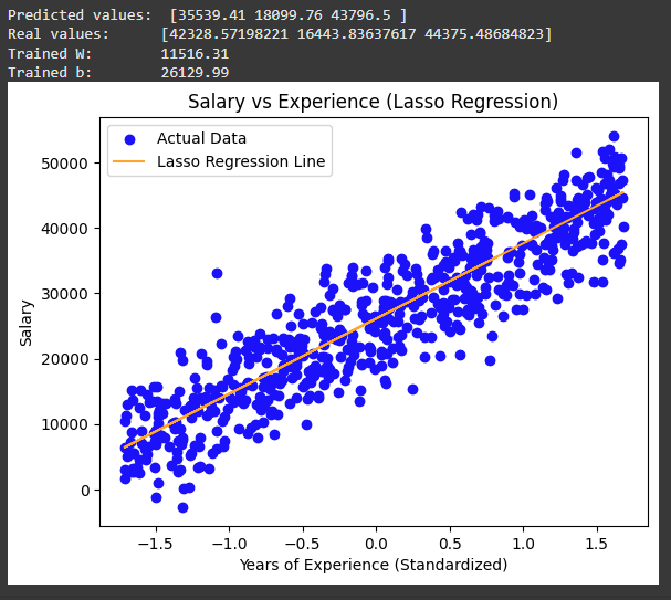
Trained Model

This output shows that the Lasso Regression model is successfully fitting the data with a clear linear relationship and it is capable of predicting salaries based on years of experience. The visualization and trained coefficients give insights into how well the model learned from the data. The close match between predicted and real values also shows the model’s ability to capture the underlying salary patterns effectively.

You can download source code from here.