Introduction to Seaborn Python (original) (raw)

Last Updated : 04 Jul, 2024

Visualization is an important part of storytelling, we can gain a lot of information from data by simply just plotting the features of data. Python provides a numerous number of libraries for data visualization, we have already seen the Matplotlib library in this article we will know about Seaborn Library.

What is Seaborn

Seaborn is an amazing visualization library for statistical graphics plotting in Python. It provides beautiful default styles and color palettes to make statistical plots more attractive. It is built on top matplotlib library and is also closely integrated with the data structures from pandas.
Seaborn aims to make visualization the central part of exploring and understanding data. It provides dataset-oriented APIs so that we can switch between different visual representations for the same variables for a better understanding of the dataset.

Different categories of plot in Seaborn

Plots are basically used for visualizing the relationship between variables. Those variables can be either completely numerical or a category like a group, class, or division. Seaborn divides the plot into the below categories –

**Relational plots: This plot is used to understand the relation between two variables.
**Categorical plots: This plot deals with categorical variables and how they can be visualized.
**Distribution plots: This plot is used for examining univariate and bivariate distributions
**Regression plots: The regression plots in Seaborn are primarily intended to add a visual guide that helps to emphasize patterns in a dataset during exploratory data analyses.
**Matrix plots: A matrix plot is an array of scatterplots.
**Multi-plot grids: It is a useful approach to draw multiple instances of the same plot on different subsets of the dataset.

Installation of Seaborn Library

For Python environment :

pip install seaborn

For conda environment :

conda install seaborn

**Dependencies for Seaborn Library

There are some libraries that must be installed before using Seaborn. Here we will list out some basics that are a must for using Seaborn.

Python 3.6 or higher
numpy (>= 1.13.3)
scipy (>= 1.0.1)
pandas (>= 0.22.0)
matplotlib (>= 2.1.2)

However, we must note that if try to use Seaborn

Some basic plots using seaborn

**Histplot: Seaborn Histplot is used to visualize the univariate set of distributions(single variable). It plots a histogram, with some other variations like kdeplot and rugplot. The Histplot function takes several arguments but the important ones are

**data: This is the array, series, or dataframe that you want to visualize. It is a required parameter.

**x: This specifies the column in the data to use for the histogram. If your data is a dataframe, you can specify the column by name.

**y: This specifies the column in the data to use for the histogram when you want to create a bivariate histogram. By default, it is set to **None, meaning that a univariate histogram will be plotted.

**bins: This specifies the number of bins to use when dividing the data into intervals for plotting. By default, it is set to “auto”, which uses an algorithm to determine the optimal number of bins.

**kde: This parameter controls whether to display a kernel density estimate (KDE) of the data in addition to the histogram. By default, it is set to **False, meaning that a KDE will not be plotted.

Python3 `

import numpy as np import seaborn as sns

sns.set(style="white")

Generate a random univariate dataset

rs = np.random.RandomState(10) d = rs.normal(size=100)

Plot a simple histogram and kde

sns.histplot(d, kde=True, color="m")

**Output:

Histogram with seaborn

**Distplot: Seaborn distplot is used to visualize the univariate set of distributions(Single features) and plot the histogram with some other variations like kdeplot and rugplot.

The function takes several parameters, but the most important ones are:

**a: This is the array, series, or list of data that you want to visualize. It is a required parameter.

**bins: This specifies the number of bins to use when dividing the data into intervals for plotting. By default, it is set to “auto”, which uses an algorithm to determine the optimal number of bins.

**kde: This parameter controls whether to display a kernel density estimate (KDE) of the data in addition to the histogram. By default, it is set to **True, meaning that a KDE will be plotted.

**hist: This parameter controls whether to display the histogram of the data. By default, it is set to **True, meaning that a histogram will be plotted.

Python `

import numpy as np import seaborn as sns

sns.set(style="white")

Generate a random univariate dataset

rs = np.random.RandomState(10) d = rs.normal(size=100)

Define the colors to use

colors = ["r", "g", "b"]

Plot a histogram with multiple colors

sns.distplot(d, kde=True, hist=True, bins=10, rug=True,hist_kws={"alpha": 0.3, "color": colors[0]}, kde_kws={"color": colors[1], "lw": 2}, rug_kws={"color": colors[2]})

**Output:

Distplot using seaborn

**Note: The distplot function has been depreciated in the newer version of the Seaborn Library

**Lineplot: The line plot is one of the most basic plots in the seaborn library. This plot is mainly used to visualize the data in the form of some time series, i.e. in a continuous manner.

Python3 `

import seaborn as sns

sns.set(style="dark") fmri = sns.load_dataset("fmri")

Plot the responses for different\

events and regions

sns.lineplot(x="timepoint", y="signal", hue="region", style="event", data=fmri)

**Output :

Lineplot using seaborn

**Lmplot: The lmplot is another most basic plot. It shows a line representing a linear regression model along with data points on the 2D space and x and y can be set as the horizontal and vertical labels respectively.

Python3 `

import seaborn as sns

sns.set(style="ticks")

Loading the dataset

df = sns.load_dataset("anscombe")

Show the results of a linear regression

sns.lmplot(x="x", y="y", data=df)

**Output :

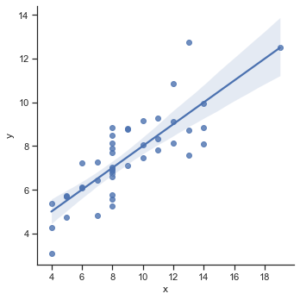
Lmplot using seaborn