Agglomerative Clustering (original) (raw)

Last Updated : 27 Nov, 2025

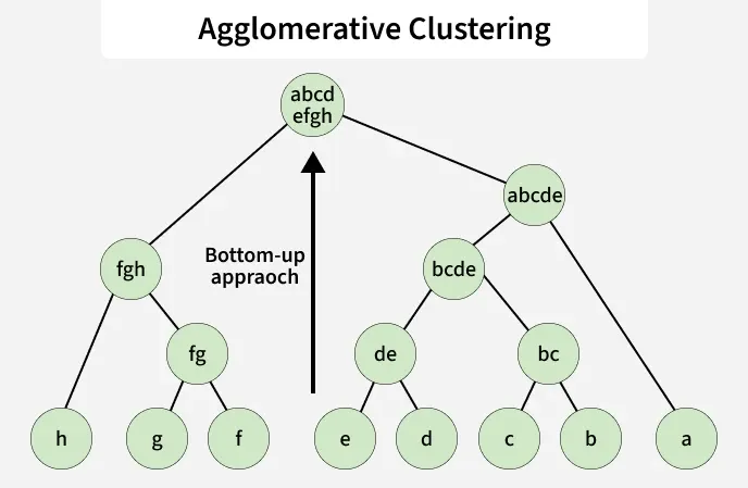
To group similar data points into clusters based on their proximity, Agglomerative Clustering is used which is a type of hierarchical clustering. It follows a bottom-up approach, where each data point starts as its own cluster and gradually merges with others based on similarity.

The merging continues until all points form a single cluster or a set number of clusters remain.
It uses distance metrics like Euclidean or Manhattan distance to measure similarity.
The process is often visualized using a dendrogram, which shows the hierarchy of cluster formation.
Common linkage methods include single, complete, average and ward linkage.

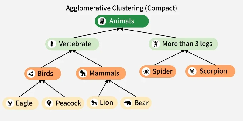
agglomerative_clustering_compact_

Animal Categorization Tree

Workflow

Lets dicuss step by step how it works:

agglomerative_clustering

Workflow of Divisive Clustering

**1. Start with all points separate:

Treat each data point as its own cluster like A, B, C, ...
Initially, you have n clusters for n data points.

**2. Compute pairwise distances:

Calculate the distance between every pair of clusters.
Common choices include Euclidean, Manhattan or Cosine distance.
Store these values in a distance matrix.

To know more about them refer to: Measures of Distance

**3. Merge the nearest clusters:

Identify the two clusters that are closest based on the chosen linkage method such as single, complete, average or Ward linkage.
Combine them into a single new cluster.

**4. Update distances:

Recalculate the distances between the newly formed cluster and all remaining clusters.
Use the same linkage rule to ensure consistency.

**5. Repeat the process:

Continue merging clusters and updating distances iteratively.
Stop when you reach a predefined number of clusters (k) or a distance threshold.

**6. Visualize the results:

Create a dendrogram to visualize how clusters merged at each step.
Choose a suitable cut on the dendrogram to obtain the final cluster groups.

Implementation

Let's see the implementation to show how agglomerative clustering works:

Step 1: Import Library

We need to import matplotlib library.

Python `

import matplotlib.pyplot as plt

Step 2: Define Leaves and Merge Sequence

List the leaf nodes (individual items) and define the bottom-up merge sequence. Each merge tuple is (left_item, right_item, parent_name).

Python `

leaves = ["Eagle", "Peacock", "Lion", "Bear", "Spider", "Scorpion"] merges = [ ("Eagle", "Peacock", "Birds"), ("Lion", "Bear", "Mammals"), ("Spider", "Scorpion", "More than 3 legs"), ("Birds", "Mammals", "Vertebrate"), ("Vertebrate", "More than 3 legs", "Animals") ]

Step 3: Build nested dictionary from merges

This creates a nested tree structure (dictionary) from the bottom-up merges. The resulting cluster_tree is a nested dict where each key maps to either a leaf string or another dict.

Python `

def build_tree_from_merges(leaves, merges): tree = {leaf: leaf for leaf in leaves} def replace_node(container, target, subtree): if isinstance(container, dict): if target in container: container[target] = subtree return True for k, v in container.items(): if replace_node(v, target, subtree): return True return False for a, b, parent in merges: subtree = { a: tree.pop(a) if a in tree else a, b: tree.pop(b) if b in tree else b } tree[parent] = subtree for top in list(tree.keys()): if top == parent: continue replace_node(tree[top], a, subtree) replace_node(tree[top], b, subtree)

root = list(tree.keys())[0]
return {root: tree[root]}

cluster_tree = build_tree_from_merges(leaves, merges)

Step 4: Compute positions

This recursive function computes (x,y) positions for every node to lay out the tree compactly. Small dx/dy values produce a compact tree.

Python `

def compute_positions(tree, x=0.0, y=0.0, dx=1.0, dy=1.0): positions = {} if isinstance(tree, dict): total_w = 0 child_centers = [] children_positions = {} for key, subtree in tree.items(): sub_pos, sub_w = compute_positions( subtree, x + total_w * dx, y - dy, dx, dy) children_positions.update(sub_pos) xs = [px for (px, py) in sub_pos.values()] center_x = sum(xs) / len(xs) child_centers.append((key, center_x)) total_w += sub_w for key, cx in child_centers: positions[key] = (cx, y) positions.update(children_positions) return positions, max(1, total_w) else: positions[tree] = (x, y) return positions, 1

positions, _ = compute_positions(cluster_tree, x=0.0, y=0.0, dx=0.9, dy=1.0)

This function walks the nested tree and returns a list of (parent, child) edges used to draw arrows.

Python `

def extract_edges(tree, parent=None): edges = [] if isinstance(tree, dict): for key, subtree in tree.items(): if parent is not None: edges.append((parent, key)) edges.extend(extract_edges(subtree, key)) return edges edges = extract_edges(cluster_tree)

Step 6: Plot the compact tree

This draws the nodes using text boxes (rounded) and arrows using ax.annotate. It sets axis limits tightly around the nodes and saves the plot to /mnt/data/agglomerative_compact.png.

Python `

def plot_compact_tree(positions, edges, leaves, title="Agglomerative Clustering"): fig, ax = plt.subplots(figsize=(8, 5)) ax.axis("off") xs = [p[0] for p in positions.values()] ys = [p[1] for p in positions.values()] xmin, xmax = min(xs) - 0.9, max(xs) + 0.9 ymin, ymax = min(ys) - 0.6, max(ys) + 0.6 ax.set_xlim(xmin, xmax) ax.set_ylim(ymin, ymax) for parent, child in edges: if parent in positions and child in positions: x_parent, y_parent = positions[parent] x_child, y_child = positions[child] ax.annotate("", xy=(x_child, y_child + 0.08), xycoords='data', xytext=(x_parent, y_parent - 0.08), textcoords='data', arrowprops=dict(arrowstyle="->", lw=1.4, color="black", shrinkA=4, shrinkB=4) ) for node, (x, y) in positions.items(): if node in leaves: face = "#fff2c2" txtcol = "black" fontsize = 10 pad = 0.25 elif node == "Animals": face = "#6e6e6e" txtcol = "white" fontsize = 11 pad = 0.32 elif node == "Vertebrate": face = "#ffd24d" txtcol = "black" fontsize = 11 pad = 0.30 else: face = "#7fd8c7" txtcol = "black" fontsize = 10 pad = 0.27 ax.text(x, y, node, ha="center", va="center", fontsize=fontsize, weight="bold" if node not in leaves else "normal", bbox=dict(boxstyle="round,pad={}".format(pad), facecolor=face, edgecolor="black")) ax.set_title(title, fontsize=14, weight="bold", pad=12) ax.text(xmin + 0.15, (ymin + ymax) / 2, "Agglomerative\nClustering\n(Bottom-Up)", ha="center", va="center", rotation=90, fontsize=9) try: out_path = "/mnt/data/agglomerative_compact.png" plt.savefig(out_path, dpi=200, bbox_inches="tight") print(f"Saved compact tree to: {out_path}") except Exception: pass plt.show() plot_compact_tree(positions, edges, leaves)

**Output:

download

Result

Real-World Applications

**Customer Segmentation (Marketing): Used to group customers based on purchase habits, browsing patterns or spending level when no predefined categories exist.
**Document & Topic Grouping (NLP / Search Engines): Clusters similar articles, research papers or news items to build topic hierarchies and recommendation systems.
**Fraud Detection (Finance & Security): Identifies unusual behavior by grouping normal patterns together and highlighting deviations as potential anomalies.
**Image Segmentation (Computer Vision): Groups pixels with similar properties like color, intensity or texture to detect objects or separate regions in an image.
**Bioinformatics & Gene Expression Analysis: Reveals hierarchical relationships between genes, proteins or species in evolutionary trees or similarity maps.

Advantages

**No Need to Predefine Number of Clusters: We don’t have to choose k beforehand. Clusters can be selected later by cutting the dendrogram at any level.
**Produces a Full Hierarchical Structure: It reveals how clusters form step-by-step, providing a clear and interpretable tree of relationships.
**Works With Any Distance Metric: Supports Euclidean, Manhattan, cosine, correlation, etc making it flexible for many types of data.
**Handles Non-Spherical and Complex Cluster Shapes: Depending on the linkage method, it can capture irregular or elongated patterns that methods like k-means cannot.