Bias and Variance in Machine Learning (original) (raw)
Last Updated : 12 Dec, 2025
Bias and Variance are two fundamental concepts that help explain a model’s prediction errors in machine learning. Bias refers to the error caused by oversimplifying a model while variance refers to the error from making the model too sensitive to training data.
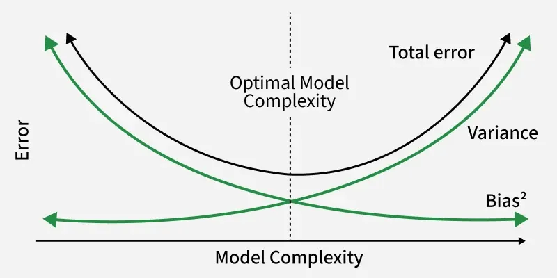
Bias Variance Tradeoff
Understanding this balance is essential for building models that generalize well to unseen data.
Bias
Bias is the error that occurs when a model is too simple to capture the true patterns in the data.
- **High bias: The model oversimplifies, misses patterns and underfits the data.
- **Low bias: The model captures patterns well and is closer to the true values.
**Example: A neural network with too few layers or neurons fails to capture complex patterns, producing consistently inaccurate outputs. This is called underfitting.
Mathematically, the formula for bias is:
\text{Bias}^2 = \big( \mathbb{E}[\hat{f}(x)] - f(x) \big)^2
Where,
- \hat{f}(x): predicted value by the model
- f(x): true value
- \mathbb{E}[\hat{f}(x)]: expected prediction over different training sets
How to Reduce Bias?
Some methods to lower bias in models are:
- **Use More Complex Models: Use models capable of capturing non-linear relationships such as neural networks or ensemble methods.
- **Add Relevant Features: Include additional informative features in the training data to give the model for capturing underlying patterns.
- **Adjust Regularization Strength: Reduce regularization to allow the model more flexibility in fitting the data.
Variance
Variance arises when a model becomes too sensitive to training data and it captures noises in data too. It fails to give prediction on unseen new data.
- **High variance: The model is too sensitive to small changes and may overfit.
- **Low variance: The model is more stable but might miss some patterns.
**Example: A deep decision tree that memorizes the training data perfectly but performs poorly on new data shows high variance, this is known as overfitting.
Mathematically, the formula for variance is:
\text{Variance} = \mathbb{E}\Big[ \big( \hat{f}(x) - \mathbb{E}[\hat{f}(x)] \big)^2 \Big]
Where,
- \hat{f}(x): predicted value by the model
- \mathbb{E}[\hat{f}(x)]: average prediction over multiple training sets
How to Reduce Variance?
Some methods to lower variance are:
- **Simplify the Model: Use a simpler model or prune overly deep decision trees to avoid overfitting.
- **Increase Training Data: Collect more data to stabilize learning and make the model generalize better.
- **Apply Regularization: Use L1 or L2 regularization to constrain model complexity and prevent overfitting.
- **Use Ensemble Methods: Implement techniques like bagging or random forests to combine multiple models and balance bias–variance trade-offs.
**Bias Variance Tradeoff
The total prediction error depends on the tradeoff between bias and variance:
| Model Type | Bias | Variance | Result |
|---|---|---|---|
| Underfitting | High | Low | Poor training and test performance |
| Optimal | Moderate | Moderate | Best generalization |
| Overfitting | Low | High | Poor test performance |
An ideal model achieves a balance of model not being too simple i.e. high bias, not too complex i.e. high variance.
Visualization
A simple way to understand bias and variance is with a dartboard analogy:
- **High Bias: Darts are clustered together but far from the target center.
- **High Variance: Darts are scattered all over the board.
- **Low Bias and Low Variance: Darts are tightly grouped near the center, showing accurate and consistent predictions.
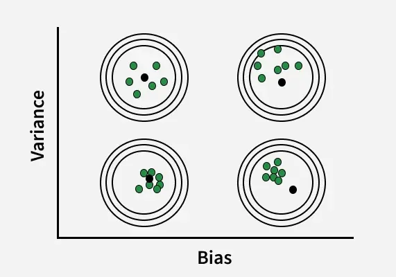
Bias-Variance Visualization
Implementation
Stepwise implementation of bias and variance calculation in Python:
Step 1: Import Libraries
Importing libraries like Numpy, Matplotlib and Scikit-learn.
Python `
import numpy as np from sklearn.linear_model import LinearRegression from sklearn.preprocessing import PolynomialFeatures from sklearn.model_selection import train_test_split import matplotlib.pyplot as plt
`
Step 2: Create Synthetic Data
Creating synthetic data using Numpy.
Python `
np.random.seed(42) X = np.linspace(0, 1, 50).reshape(-1, 1) y = np.sin(2 * np.pi * X).ravel() + np.random.normal(0, 0.2, 50)
`
Step 3: Splitting the Data
Splitting the data into X_train, X_test, y_train, y_test.
Python `
X_train, X_test, y_train, y_test = train_test_split(X, y, test_size=0.3, random_state=42)
`
Step 4: Compute Bias, Variance and Error
Defining function to compute bias, variance and error.
- Training the model on random samples multiple times.
- Calculating mean prediction, bias² and variance.
- Adding them to get total error. Python `
def bias_variance_error_bootstrap(model, X_train, y_train, X_test, y_test, runs=30): preds = [] n = X_train.shape[0] for _ in range(runs): idx = np.random.choice(n, n, replace=True) X_sample = X_train[idx] y_sample = y_train[idx] preds.append(model.fit(X_sample, y_sample).predict(X_test))
preds = np.array(preds)
y_pred_mean = preds.mean(axis=0)

bias_sq = ((y_test - y_pred_mean)**2).mean()
variance = preds.var(axis=0).mean()
total_error = bias_sq + variance

return bias_sq, variance, total_error
`
Step 5: Linear Regression (High Bias)
Linear regression has high bias because it’s too simple and underfits, missing complex patterns.
- Training a Linear Regression model on training data.
- Using bootstrap sampling to estimate bias², variance and total error.
- Printing the bias, variance and total error values for analysis. Python `
lin_model = LinearRegression() b_lin, v_lin, e_lin = bias_variance_error_bootstrap(lin_model, X_train, y_train, X_test, y_test) print(f"Linear Regression -> Bias^2: {b_lin:.3f}, Variance: {v_lin:.3f}, Total Error: {e_lin:.3f}")
`
**Output:
Linear Regression -> Bias^2: 0.218, Variance: 0.014, Total Error: 0.232
Step 6: Polynomial Regression (High Variance)
Polynomial regression has high variance because it’s too flexible and overfits, capturing noise in the data.
- Transforming the data into polynomial features for higher model complexity.
- Fitting a Linear Regression model on the transformed data.
- Calculating bias², variance and total error using bootstrap sampling.
- Displaying the results to compare with the linear model. Python `
poly = PolynomialFeatures(degree=10) X_train_poly = poly.fit_transform(X_train) X_test_poly = poly.transform(X_test) poly_model = LinearRegression() b_poly, v_poly, e_poly = bias_variance_error_bootstrap(poly_model, X_train_poly, y_train, X_test_poly, y_test) print(f"Polynomial Regression -> Bias^2: {b_poly:.3f}, Variance: {v_poly:.3f}, Total Error: {e_poly:.3f}")
`
**Output:
Polynomial Regression -> Bias^2: 0.043, Variance: 0.416, Total Error: 0.459
Step 7: Visualize
Visualizing linear regression and polynomial regression using scatter plot.
Python `
plt.scatter(X, y, label="Data", color='blue') plt.plot(X_test, lin_model.fit(X_train, y_train).predict(X_test), color='red', label="Linear Regression") plt.scatter(X_test, poly_model.fit(X_train_poly, y_train).predict(X_test_poly), color='green', label="Polynomial Regression", s=20) plt.title("Bias vs Variance: Linear vs Polynomial Regression") plt.legend() plt.show()
`
**Output:
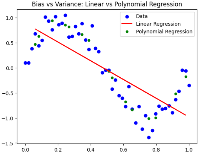
Graph
You can download the source code from here.
Applications
Some of the applications of bias and variance analysis are:
- **Model Selection: Helps determine whether a simple or complex model is best suited for the task ensuring good generalization.
- **Hyperparameter Tuning: Guides fine tuning parameters such as learning rate, regularization strength or tree depth to reduce errors.
- **Model Evaluation: Assists in identifying underfitting or overfitting by comparing training and test performance.
- **Error Analysis: Helps pinpoint the main causes of prediction errors and refine model strategies accordingly.
- **Ensemble Learning: Balances bias and variance effectively by combining multiple models to enhance stability and accuracy.
Advantages
Some of the advantages of understanding bias and variance are:
- **Improves Model Accuracy: Enables building models that perform consistently well on unseen data.
- **Supports Efficient Training: Saves computational resources by avoiding unnecessarily complex or overfitted models.
- **Enhances Interpretability: Makes it easier to understand and explain the reasons behind model errors.
- **Guides Model Complexity: Helps find the optimal level of model complexity for different data sizes and problems.
Limitations
Some of the limitations of bias and variance concepts are:
- **Difficult to Quantify Precisely: Measuring exact bias and variance in modern complex models can be challenging.
- **Highly Data Dependent: Model behavior may vary significantly across datasets with different characteristics.
- **Unpredictable in Deep Learning: Deep neural networks can display unexpected bias-variance dynamics due to non-convex optimization.
- **Tradeoff Challenge: Minimizing one often increases the other requiring careful experimentation and balance.