Binary classification using LightGBM (original) (raw)

Last Updated : 6 Sep, 2025

LightGBM (Light Gradient Boosting Machine) is an open-source gradient boosting framework designed for efficient and scalable machine learning. It is widely used for classification tasks, including binary classification and is optimized for speed and memory usage.

We will implement binary classification using LightGBM:

1. Installing Libraries

We will install LightGBM for classification tasks.

pip install lightgbm

2. Importing Libraries and Dataset

We will import the necessary Python libraries such as pandas, numpy, seaborn, matplotlib, sklearn and load the dataset.

You can download dataset from here.

Python `

import pandas as pd import numpy as np import seaborn as sb import matplotlib.pyplot as plt import lightgbm as lgb from sklearn.preprocessing import StandardScaler from sklearn.model_selection import train_test_split from sklearn.metrics import roc_auc_score from lightgbm import LGBMClassifier import warnings warnings.filterwarnings('ignore')

df = pd.read_csv('/content/diabetes.csv')

`

2.1. Previewing the Dataset

We will check the first few rows to understand the data structure.

• **df.head() displays the first five rows for a quick preview Python `

df.head()

`

**Output:

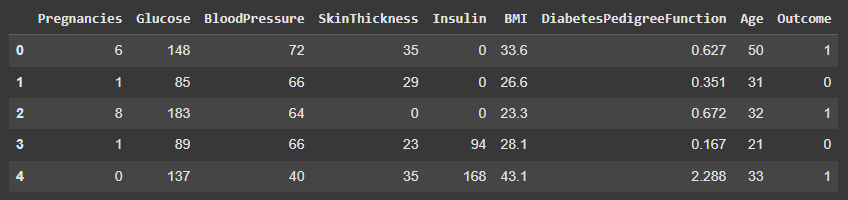
Previewing the Dataset

2.2. Dataset Shape

We will check the dimensions of the dataset.

• **df.shape returns the number of rows and columns Python `

df.shape

`

**Output:

(768, 9)

2.3. Dataset Information

We will check the data types and null values.

• **df.info() shows column data types and counts of non-null values Python `

df.info()

`

**Output:

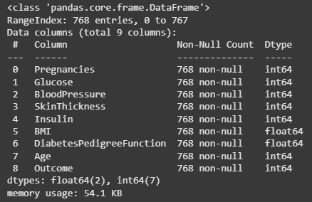
Dataset Information

2.4. Descriptive Statistics

We will compute statistical summaries of numeric features.

• **df.describe() shows count, mean, std, min, max and percentiles Python `

df.describe()

`

**Output:

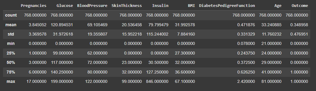
Descriptive Statistics

3. Exploratory Data Analysis (EDA)

We will analyze patterns, distributions and relationships among features.

3.1. Class Distribution

We will visualize the distribution of the target variable Outcome.

• **value_counts() counts frequency of each class.
• **plt.pie() plots a pie chart; autopct='%1.1f%%' shows percentages.
• It helps identify class imbalance which can affect model training. Python `

temp = df['Outcome'].value_counts() plt.pie(temp.values, labels=temp.index.values, autopct='%1.1f%%') plt.title("Class Distribution") plt.show()

`

**Output:

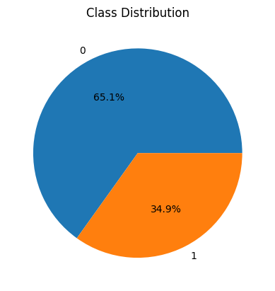
Class Distribution

3.2. Correlation Matrix

We will check correlations between features.

• **df.corr() computes pairwise correlations of columns.
• **sb.heatmap() visualizes correlation matrix and **annot=True shows values.
• Useful for detecting highly correlated features (>0.7) which may indicate redundancy or risk of data leakage. Python `

sb.heatmap(df.corr() > 0.7, cbar=False, annot=True) plt.show()

`

**Output:

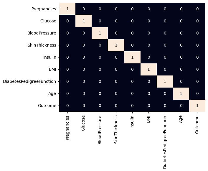
Correlation Matrix

3.3. Feature Distributions

We will visualize individual feature's distributions.

• **plt.figure(figsize=(15, 15)) sets the size of the figure for all subplots.
• **plt.subplot(nrows, ncols, index) specifies the position of the subplot in the grid.
• **sb.histplot(df[col], kde=True) plots a histogram with a KDE (Kernel Density Estimate) to show distribution.
• **plt.tight_layout() automatically adjusts subplot spacing to prevent overlap.
• Visualizing distributions helps detect skewness, spread and outliers in numerical features. Python `

num_cols = ['Pregnancies', 'Glucose', 'BloodPressure', 'SkinThickness', 'Insulin', 'BMI', 'DiabetesPedigreeFunction', 'Age']

plt.figure(figsize=(15, 15)) for col in num_cols: plt.subplot(3, 3, num_cols.index(col)+1) sb.histplot(df[col], kde=True)

plt.tight_layout() plt.show()

`

**Output:

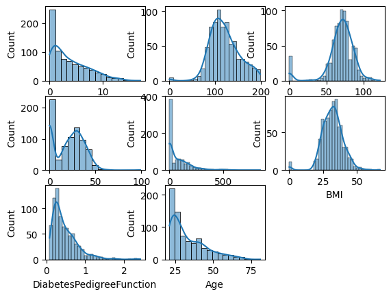
Feature Distributions

3.4. Count Plots

We will visualize categorical feature relationships with the target.

• **countplot() displays counts for each category; hue separates by target variable.
• Helps observe trends between features and target variable. Python `

sb.countplot(data=df, x='Pregnancies', hue='Outcome') plt.show()

`

**Output:

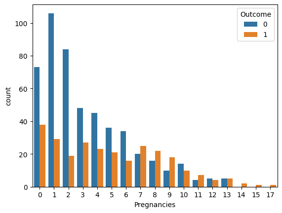
Count Plots

Insights from the Diabetes dataset:

• The dataset is imbalanced: fewer positive cases (Outcome=1) than negative cases.
• Features like Glucose, BMI and Age show skewed distributions and may influence the target strongly.
• Higher Pregnancies tend to correlate with a higher likelihood of diabetes.
• Most other features show weak correlations with each other (no multicollinearity issues).
• Skewed or zero-heavy features (like Insulin and SkinThickness) might benefit from transformations.

4. Data Preprocessing

We will prepare the dataset for LightGBM.

4.1. Splitting Features and Target

We will split the dataset into input features and target variable.

• **drop('Outcome', axis=1) removes target column to create features.
• **train_test_split() splits data into training and validation sets.
• **test_size=0.2 reserves 20% of data for validation.
• **random_state=2023 ensures reproducibility. Python `

features = df.drop('Outcome', axis=1) target = df['Outcome']

X_train, X_val, Y_train, Y_val = train_test_split( features, target, test_size=0.2, random_state=2023 )

`

4.2. Feature Scaling

We will standardize the features to improve model learning.

• **StandardScaler() transforms features to mean=0, std=1.
• **fit_transform() computes mean or standard deviation (std) on training data and transforms it.
• **transform() applies the same scaling to validation data.
• Standardization improves gradient boosting model performance. Python `

scaler = StandardScaler() X_train = scaler.fit_transform(X_train) X_val = scaler.transform(X_val)

`

5. Dataset Preparation for LightGBM

We will convert arrays into LightGBM dataset objects for training.

• **lgb.Dataset() prepares dataset compatible with LightGBM.
• label specifies target variable.
• reference ensures validation set is consistent with training set. Python `

train_data = lgb.Dataset(X_train, label=Y_train) test_data = lgb.Dataset(X_val, label=Y_val, reference=train_data)

`

6. Binary Classification Model Using LightGBM

We will define model parameters and train the classifier.

• **objective='binary' defines task as binary classification.
• **metric='auc' uses ROC-AUC as evaluation metric.
• **boosting_type='gbdt' uses Gradient Boosting Decision Tree algorithm.
• **num_leaves=31 sets max number of leaves per tree.
• **learning_rate=0.05 sets step size for boosting.
• **feature_fraction=0.9 specifies fraction of features per iteration.
• **early_stopping_rounds=10 stops training if no improvement. Python `

params = { 'objective': 'binary', 'metric': 'auc', 'boosting_type': 'gbdt', 'num_leaves': 31, 'learning_rate': 0.05, 'feature_fraction': 0.9 }

num_round = 100 bst = lgb.train(params, train_data, num_round, valid_sets=[test_data], early_stopping_rounds=10)

`

**Output:

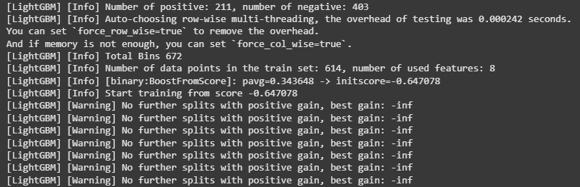
Binary Classification Model Using LightGBM

7. Prediction and Evaluation

We will generate predictions and evaluate performance using ROC-AUC.

• **bst.predict() predicts probabilities for each instance.
• ****(y > 0.5).astype(int)** converts probabilities to binary outcomes.
• **roc_auc_score() computes ROC-AUC score for evaluation. Python `

y_train = bst.predict(X_train) y_val = bst.predict(X_val)

y_train_class = (y_train > 0.5).astype(int) y_val_class = (y_val > 0.5).astype(int)

print("Training ROC-AUC: ", ras(Y_train, y_train)) print("Validation ROC-AUC: ", ras(Y_val, y_val))

`

**Output:

Training ROC-AUC: 1.0
Validation ROC-AUC: 0.6791463194067643