Central Limit Theorem in Data Science and Data Analytics (original) (raw)
Last Updated : 8 Dec, 2025
The Central Limit theorem says that if we take many random samples from any population and calculate their averages, those averages will form a bell-shaped (normal) curve even if the original data is not normally distributed as long as the sample size is large enough. This helps us make predictions about the whole population using just sample data.
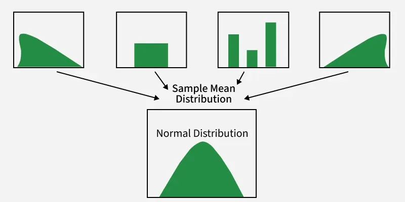
Normal Distribution
By calculating sample means these averages will tend to form a normal distribution. This normality holds true as long as the sample size is sufficiently large, typically n ≥ 30 providing the foundation for making inferences about populations even when we don’t have access to all the data.
Central Limit Theorem Formula
You have a population where the data follows some random variable X and this population has:
- **Mean \mu the average of the population
- **Standard deviation \sigma
let’s say we take a sample of size n from this population and calculate its mean \bar{X} then the Z-Score is given below:
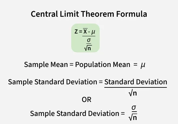
Central Limit Theorem Formula
As the sample size increases the distribution of sample means becomes more concentrated around \mu and resembles a normal distribution.
**Key Assumptions for Central Limit Theorem
For the Central Limit Theorem (CLT) to work properly, a few conditions must be met:
- **Random Sampling: The sample must be chosen randomly to fairly represent the whole population.
- **Independence: Each data point should be independent one should not influence another.
- **Large Enough Sample Size: A sample size of at least 30 is usually enough for the sample mean to follow a normal distribution.
- **Finite Mean and Variance: The population should have a defined average and variation extreme or unlimited values can make CLT unreliable.
By ensuring these assumptions are met. The theorem can be used to draw conclusions about the population.
While working with CLT we often need to work with skwed data, to learn more about skwed data refer to:**Skewness
How CLT works in Data Science
You are data analyst at a tech company. Users around the world have different web page load times, usually being biased based on network speed and location. you need to estimate the mean load time but it is impractical to verify every user.
Let's solve this problem step-by-step:
**Step 1: Problem Identification
Instead of analyzing all user , you take a small sample (e.g., 50 users) to estimate the average load time. But since the data isn’t normally distributed, can you trust this average? This is where the Central Limit Theorem comes into play.
**Step 2: Data Sampling Process
To use the Central Limit Theorem (CLT):
- Take 50 random users and calculate their mean load time.
- Do it 1,000 times to obtain 1,000 sample means.
- When you graph these means, the outcome is an approximately normal distribution even though the original data is skewed.
**Step 3: How to Implement the CLT
Now that we understand the scenario let us walk through the steps of how to implement the Central Limit Theorem using Python. Before its implementation we should have some basic knowledge about numpy and matplotlib.
We will generate fake web load times using an exponential distribution (to represent skewed data), take many random samples, and plot their means to observe how they form a normal distribution.
Python `
import numpy as np import matplotlib.pyplot as plt
Simulate skewed load time data
np.random.seed(0) population = np.random.exponential(scale=2.0, size=100000)
Parameters
sample_size = 50 num_samples = 1000 sample_means = []
Take samples and compute means
for _ in range(num_samples): sample = np.random.choice(population, size=sample_size) sample_means.append(np.mean(sample))
Plot the sample means
plt.hist(sample_means, bins=40, color='skyblue', edgecolor='black') plt.title('Sampling Distribution of Web Page Load Time (Means)') plt.xlabel('Sample Mean Load Time') plt.ylabel('Frequency') plt.grid(True) plt.show()
`
**Output:
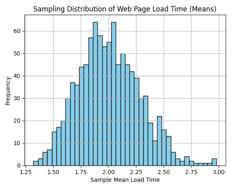
Sampling distribution
Although the original load time data is skewed, the histogram of sample means shows a normal curve. This confirms the Central Limit Theorem even non-normal data can produce a normal sampling distribution when you take enough samples.
**Practical Applications of the Central Limit Theorem
The Central Limit Theorem (CLT) is widely used in machine learning and data analysis:
- Model Evaluation and Confidence Intervals: CLT helps build confidence intervals around model predictions, showing how reliable they are more data leads to tighter intervals and more trust in results.
- **A/B Testing: A/B Testing is used in product development, CLT ensures that average outcomes from repeated experiments become normally distributed, even with skewed data.
- **Error and Uncertainty Estimation: CLT allows us to estimate prediction errors and standard errors, helping assess model uncertainty on new data.
- **Bootstrapping: By resampling data, CLT supports reliable estimation of metrics like MSE and confidence intervals for model parameters.
- **Feature Importance: CLT helps check if feature rankings remain stable across samples, ensuring the most consistent and reliable features are chosen.
Limitations of Central Limit Theorem
The Central Limit Theorem (CLT) is a useful concept in statistics but it come with some limitations that are important to understand. Let's understand them one by one:
- **Sample Size: CLT is efficient for large samples. CLT will not work with very small samples, particularly with data that is skewed, and the mean will not follow a normal distribution and may result in erroneous conclusions.
- **Population Shape: While CLT can apply to any population, if the data is very uneven or has extreme values, you’ll need a much larger sample for the average to become normal.
- **Independent Data: The data points in your sample must be independent. This isn’t true for things like time series data, where one value depends on the previous one, which can affect the results.
- **Random Sampling: The sample needs to be selected randomly. If it is biased (e.g., only sample from a specific group), then it won't accurately represent the entire population, and CLT won't function as intended.
- **Finite Variance: The population should have a well-defined limited range in values. If variation is infinite or too large, then CLT does not apply.