Classifying data using Support Vector Machines(SVMs) in Python (original) (raw)

Last Updated : 2 Aug, 2025

Support Vector Machines (SVMs) are supervised learning algorithms widely used for classification and regression tasks. They can handle both linear and non-linear datasets by identifying the optimal decision boundary (hyperplane) that separates classes with the maximum margin. This improves generalization and reduces misclassification.

Core Concepts

• **Hyperplane : The decision boundary separating classes. It is a line in 2D, a plane in 3D or a hyperplane in higher dimensions.
• **Support Vectors : The data points closest to the hyperplane. These points directly influence its position and orientation.
• **Margin : The distance between the hyperplane and the nearest support vectors from each class. SVMs aim to maximize this margin for better robustness and generalization.
• **Regularization Parameter (C) : Controls the trade-off between maximizing the margin and minimizing classification errors. A high value of C prioritizes correct classification but may overfit. A low value of C prioritizes a larger margin but may underfit.

Optimization Objective

SVMs solve a constrained optimization problem with two main goals:

1. Maximize the margin between classes for better generalization.
2. Minimize classification errors on the training data, controlled by the parameter C.

The Kernel Trick

Real-world data is rarely linearly separable. The kernel trick elegantly solves this by implicitly mapping data into higher-dimensional spaces where linear separation becomes possible, without explicitly computing the transformation.

Common Kernel Functions

• **Linear Kernel: Ideal for linearly separable data, offers the fastest computation and serves as a reliable baseline.
• **Polynomial Kernel: Models polynomial relationships with complexity controlled by degree d, allowing curved decision boundaries.
• **Radial Basis Function (RBF) Kernel: Maps data to infinite-dimensional space, widely used for non-linear problems with parameter \gamma controlling influence of each sample.
• **Sigmoid Kernel: Resembles neural network activation functions but is less common in practice due to limited effectiveness.

Implementing SVM Classification in Python

1. Importing Required Libraries

We will import required python libraries

• **NumPy: Used for numerical operations.
• **Matplotlib: Used for plotting graphs (can be used later for decision boundaries).
• **load_breast_cancer: Loads the Breast Cancer Wisconsin dataset from scikit-learn.
• **StandardScaler: Standardizes features by removing the mean and scaling to unit variance.
• **SVC: Support Vector Classifier from scikit-learn. Python `

import numpy as np import matplotlib.pyplot as plt from sklearn.datasets import load_breast_cancer from sklearn.model_selection import train_test_split from sklearn.preprocessing import StandardScaler from sklearn.svm import SVC from sklearn.metrics import accuracy_score, classification_report

`

2. Loading the Dataset

We will load the dataset and select only two features for visualization:

• **load_breast_cancer(): Returns a dataset with 569 samples and 30 features.
• **data.data[:, [0, 1]]: Selects only two features (mean radius and mean texture) for simplicity and visualization.
• **data.target: Contains the binary target labels (malignant or benign). Python `

data = load_breast_cancer() X = data.data[:, [0, 1]] y = data.target

`

3. Splitting the Data

We will split the dataset into training and test sets:

• **train_test_split: splits data into training (80%) and test (20%) sets
• **random_state=42: ensures reproducibility Python `

X_train, X_test, y_train, y_test = train_test_split( X, y, test_size=0.2, random_state=42 )

`

4. Scale the Features

We will scale the features so that they are standardized:

• **StandardScaler – standardizes data by removing mean and scaling to unit variance
• **fit_transform() – fits the scaler to training data and transforms it
• **transform() – applies the same scaling to test data Python `

scaler = StandardScaler() X_train_scaled = scaler.fit_transform(X_train) X_test_scaled = scaler.transform(X_test)

`

5. Train the SVM Classifier

We will train the Support Vector Classifier:

• **SVC: creates an SVM classifier with a specified kernel
• **kernel='linear': uses a linear kernel for classification
• **C=1.0: regularization parameter to control margin vs misclassification
• **fit(): trains the classifier on scaled training data Python `

svm_classifier = SVC(kernel='linear', C=1.0, random_state=42) svm_classifier.fit(X_train_scaled, y_train)

`

6. Evaluate the Model

We will predict labels and evaluate model performance:

• **predict(): makes predictions on test data
• **accuracy_score(): calculates prediction accuracy
• **classification_report(): shows precision, recall and F1-score for each class Python `

y_pred = svm_classifier.predict(X_test_scaled) print(f"Accuracy: {accuracy_score(y_test, y_pred):.2f}") print(classification_report(y_test, y_pred, target_names=data.target_names))

`

**Output:

SVM - output

Visualizing the Decision Boundary

We will plot the decision boundary for the trained SVM model:

• **np.meshgrid() : creates a grid of points across the feature space
• **predict() : classifies each point in the grid using the trained model
• **plt.contourf() : fills regions based on predicted classes
• **plt.scatter() : plots the actual data points Python `

def plot_decision_boundary(X, y, model, scaler): h = 0.02 # Step size for mesh x_min, x_max = X[:, 0].min() - 1, X[:, 0].max() + 1 y_min, y_max = X[:, 1].min() - 1, X[:, 1].max() + 1 xx, yy = np.meshgrid(np.arange(x_min, x_max, h), np.arange(y_min, y_max, h))

# Predict on mesh points
Z = model.predict(scaler.transform(np.c_[xx.ravel(), yy.ravel()]))
Z = Z.reshape(xx.shape)

# Plot decision boundary and data points
plt.contourf(xx, yy, Z, cmap=plt.cm.coolwarm, alpha=0.3)
plt.scatter(X[:, 0], X[:, 1], c=y, cmap=plt.cm.coolwarm, edgecolors='k')
plt.xlabel(data.feature_names[0])
plt.ylabel(data.feature_names[1])
plt.title('SVM Decision Boundary')
plt.show()

plot_decision_boundary(X_train, y_train, svm_classifier, scaler)

`

**Output:

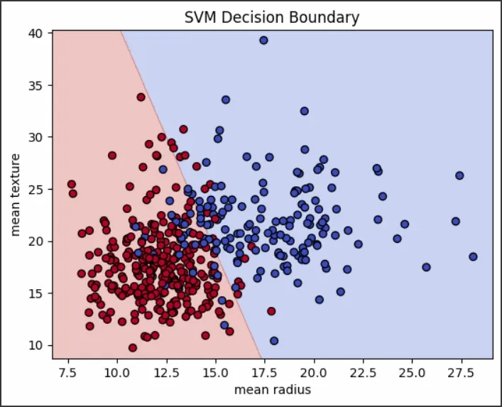
SVM decision boundary

Why Use SVMs

SVMs work best when the data has clear margins of separation, when the feature space is high-dimensional (such as text or image classification) and when datasets are moderate in size so that quadratic optimization remains feasible.

Advantages

• Performs well in high-dimensional spaces.
• Relies only on support vectors, which speeds up predictions.
• Can be used for both binary and multi-class classification.

Limitations

• Computationally expensive for large datasets with time complexity O(n²)–O(n³).
• Requires feature scaling and careful hyperparameter tuning.
• Sensitive to outliers and class imbalance, which may skew the decision boundary.

Support Vector Machines are a robust choice for classification, especially when classes are well-separated. By maximizing the margin around the decision boundary, they deliver strong generalization performance across diverse datasets.

Performance Optimization Tips

For Large Datasets

• Use LinearSVC for linear kernels (faster than SVC with linear kernel)
• Consider SGDClassifier with hinge loss as an alternative

Memory Management

• Use probability = False if you don't need probability estimates
• Consider incremental learning for very large datasets
• Use sparse data formats when applicable

Preprocessing Best Practices

• Always scale features before training
• Remove or handle outliers appropriately
• Consider feature engineering for better separability
• Use dimensionality reduction for high-dimensional sparse data