Handwritten Digit Recognition using Neural Network (original) (raw)

Last Updated : 23 Jul, 2025

Handwritten digit recognition is a classic problem in machine learning and computer vision. It involves recognizing handwritten digits (0-9) from images or scanned documents. This task is widely used as a benchmark for evaluating machine learning models especially neural networks due to its simplicity and real-world applications such as postal code recognition and bank check processing. In this article we will implement Handwritten Digit Recognition using Neural Network.

Let’s implement the solution step-by-step using Python and TensorFlow/Keras.

Step 1: Import Libraries

Before starting, we need to import the necessary libraries for data manipulation, visualization, and model building. We will use numpy, matplotlib, scikit learn and tenserflow.

Python `

import numpy as np import pandas as pd import matplotlib.pyplot as plt from sklearn.model_selection import train_test_split from tensorflow.keras.models import Sequential from tensorflow.keras.layers import Dense, Flatten from tensorflow.keras.utils import to_categorical

`

Step 2: Load and Explore the Dataset

We will load the dataset and inspect its structure to understand the features and labels. You can download this dataset from **here.

• The dataset contains 42,000 rows where each row represents an image.
• The first column (label) indicates the digit (0-9) and the remaining columns represent pixel values of the image.
• We separate these into X (pixel values) and y (labels).
• X has 42,000 samples with 784 features (28x28 pixels) and y has 42,000 labels. Python `

train_data = pd.read_csv('/content/Train.csv') print("Shape of train_data:", train_data.shape)

X = train_data.iloc[:, 1:]
y = train_data.iloc[:, 0]

print("Shape of X after separating features:", X.shape)

`

**Output:

Shape of train_data: (42000, 785)
Shape of X after separating features: (42000, 784)

Step 3: Preprocess the Data

Raw data often needs cleaning and formatting before it can be fed into a neural network. Let’s preprocess the data to make it ready for training.

• First we ensure X is in the correct format (Pandas DataFrame).
• Then we convert all pixel values to numeric format and replace any missing values with 0.
• Next we normalize the pixel values to the range [0, 1] by dividing them by 255.0. This helps the model learn faster.
• Finally we reshape the data to include a channel dimension making it compatible with neural networks. Python `

if not isinstance(X, pd.DataFrame): X = pd.DataFrame(X) X = X.apply(pd.to_numeric, errors='coerce') X = X.fillna(0)
X = X.values / 255.0 X = X.reshape(-1, 28, 28, 1) print("Shape of X after reshaping:", X.shape)

`

**Output

Shape of X after reshaping: (42000, 28, 28, 1)

Step 4: One-Hot Encode the Labels

Neural networks work best when labels are in a specific format called "one-hot encoding." Let’s convert our labels into this format.

Python `

y = to_categorical(y, num_classes=10) print("Shape of y after one-hot encoding:", y.shape)

`

**Output:

Shape of y after one-hot encoding: (42000, 10)

Step 5: Split the Data

To evaluate our model effectively we need to split the data into a training set and a validation set. Here we will use 80% data for training rest for testing.

Python `

X_train, X_val, y_train, y_val = train_test_split(X, y, test_size=0.2, random_state=42) print("X_train shape:", X_train.shape)

`

**Output:

X_train shape: (33600, 28, 28, 1)

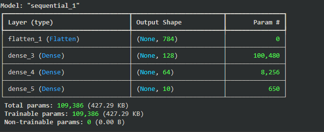
Step 6: Build the Neural Network Model

Now let’s define the architecture of our neural network. We define a simple feedforward neural network with three layers:

• A Flatten layer converts the 28x28 image into a single vector of length 784.
• Two hidden layers with 128 and 64 neurons use the ReLU activation function to introduce non-linearity.
• An output layer with 10 neurons uses the softmax activation function to predict probabilities for each digit (0-9).
• We compile the model with the Adam optimizer, categorical cross-entropy loss, and accuracy as the evaluation metric. Python `

model = Sequential([ Input(shape=(28, 28, 1)), Flatten(), Dense(128, activation='relu'), Dense(64, activation='relu'), Dense(10, activation='softmax') ]) model.compile(optimizer='adam', loss='categorical_crossentropy', metrics=['accuracy']) model.summary()

`

**Output:

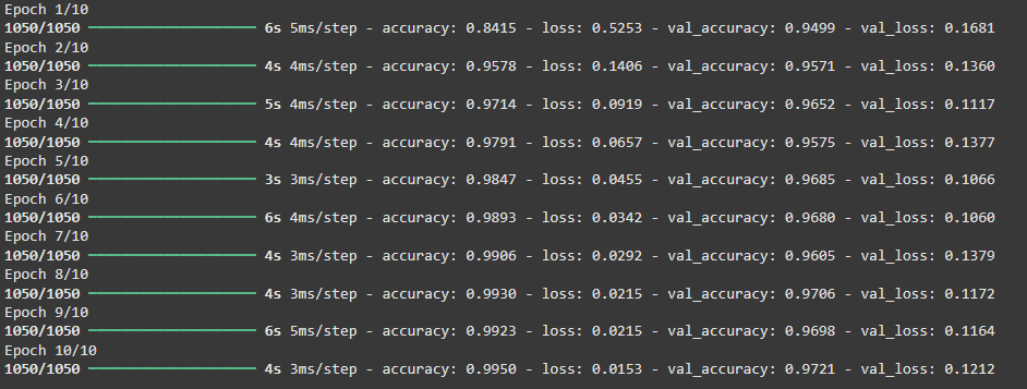
Step 7: Train the Model

With the model defined it’s time to train it on the training data. The model trains for 10 iterations (epochs) over the entire training dataset. During training it processes the data in batches of 32 samples for efficiency.

Python `

history = model.fit(X_train, y_train, epochs=10, batch_size=32, validation_data=(X_val, y_val))

`

**Output:

Step 8: Evaluate the Model

Once training is complete we evaluate the model’s performance on the validation set and plot the training and validation accuracy to see how well the model learned over time. This helps us identify issues like overfitting.

Python `

val_loss, val_accuracy = model.evaluate(X_val, y_val) print(f"Validation Accuracy: {val_accuracy * 100:.2f}%") plt.plot(history.history['accuracy'], label='Training Accuracy') plt.plot(history.history['val_accuracy'], label='Validation Accuracy') plt.legend() plt.show()

`

**Output:

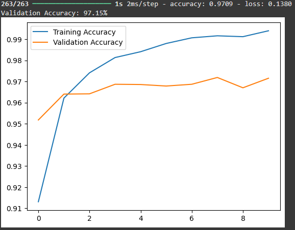
The blue line represents the **training accuracy which consistently increases over the training steps while the orange line represents the **validation accuracy which fluctuates slightly but shows a positive trend. By the end of the training the model achieves a training accuracy of around 96.81% and a validation accuracy of 97.13% indicating the model performs well on both training and validation data suggesting good generalization capability.

Step 9: Make Predictions

Let’s use the trained model to make predictions on new data. We load the test data preprocess it similarly to the training data and feed it into the model to get predictions. You can download the test dataset from **here****.**

Python `

test_data = pd.read_csv('/content/test.csv') X_test = test_data.values / 255.0 X_test = X_test.reshape(-1, 28, 28, 1) predictions = model.predict(X_test) predicted_labels = np.argmax(predictions, axis=1) for i in range(5): plt.imshow(X_test[i].reshape(28, 28), cmap='gray') plt.title(f"Predicted: {predicted_labels[i]}") plt.axis('off') plt.show()

`

**Output:

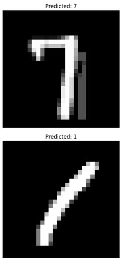
Our model is working fine making right predictions.

By using neural network architecture we were able to train the model on a dataset of 42,000 handwritten digits achieving impressive accuracy. The model successfully generalized making it capable of recognizing unseen digits effectively. This process showcases the potential of machine learning algorithms in solving real-world problems involving image recognition.

Get Source code from here:**click here****.**