Implementing gradient descent in Python to find a local minimum (original) (raw)

Last Updated : 25 Oct, 2025

Gradient Descent is an optimization algorithm used to find the local minimum of a function. It is used in machine learning to minimize a cost or loss function by iteratively updating parameters in the opposite direction of the gradient. It works by calculating the derivative i.e slope of a function and moving in the direction opposite to the slope to reach a minimum. It can be applied to any differentiable function.

Gradient Descent

Mathematical Concept

The mathematical formula for Gradient Descent:

x_{\text{new}} = x_{\text{old}} - \alpha \cdot f'(x)

Where:

• x_{\text{new}} is the current value of the variable
• \alpha is the learning rate
• x_{\text{old}} is the derivative of the function

The derivative points in the direction of the steepest ascent. By moving in the opposite direction, we approach the local minimum.

Implementation

Here’s an example to find the minimum of f(x) = x^2 + 4x + 4.

Step 1: Importing Libraries

Importing libraries like Numpy and Matplotlib.

Python `

import numpy as np import matplotlib.pyplot as plt

`

Step 2: Minimize Function

Defining function to minimize.

Python `

def f(x): return x*2 + 4x + 4

`

Step 3: Derivative

Finding derivative of the function.

Python `

def df(x): return 2*x + 4

`

Step 4: Gradient Descent

Implementing Gradient Descent.

Python `

def gradient_descent(starting_point, learning_rate, iterations): x = starting_point for i in range(iterations): x = x - learning_rate * df(x) # update step print(f"Iteration {i+1}: x = {x:.4f}, f(x) = {f(x):.4f}") return x

starting_point = 0 learning_rate = 0.1 iterations = 10

minimum = gradient_descent(starting_point, learning_rate, iterations) print(f"\nLocal minimum occurs at x = {minimum:.4f}, f(x) = {f(minimum):.4f}")

`

**Output:

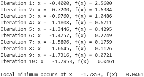
Local Minimum

Step 5: Visualizing

Visualizing using Matplotlib.

Python `

x_vals = np.linspace(-10, 2, 100) y_vals = f(x_vals) plt.plot(x_vals, y_vals, label="f(x) = x^2 + 4x + 4") plt.scatter(minimum, f(minimum), color='red', label="Local Minimum") plt.xlabel("x") plt.ylabel("f(x)") plt.title("Gradient Descent Visualization") plt.legend() plt.show()

`

**Output:

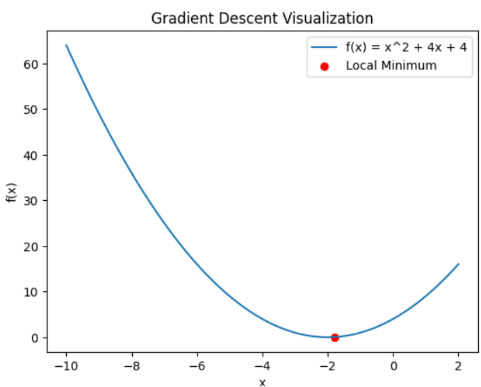
Graph

Here the red dot shows the local minimum reached by gradient descent.

Applications

1. **Machine Learning: Optimizes linear and logistic regression models by minimizing cost functions helping models learn optimal parameters.
2. **Deep Learning: Trains neural networks by adjusting weights and biases to minimize loss enabling models to learn complex patterns.
3. **Economics and Finance: Used for optimization tasks like minimizing costs, maximizing profits or portfolio optimization.
4. **Physics and Engineering: Solves systems where minima represent stable states such as energy optimization or mechanical design.
5. **Computer Vision: Optimizes models for tasks like image recognition and object detection improving performance in classification and segmentation.

Advantages

1. **Simple to Implement: Easy to code and understand, suitable for beginners and professionals.
2. **Flexible: Works for functions with one or multiple variables across many optimization problems.
3. **Widely Used: Core method in machine learning and deep learning for training models.
4. **Efficient for Large Problems: Mini-batch or stochastic versions handle large datasets effectively while saving computation time.
5. **Iterative Improvement: Gradually improves parameters giving control over convergence and model refinement.

Limitations

1. **May Converge to Local Minimum: In non-convex functions, it can get trapped in a local minimum or saddle point instead of reaching the global minimum.
2. **Sensitive to Learning Rate: A high learning rate may overshoot the minimum, while a low one makes convergence very slow.
3. **Can Be Slow for Large Datasets: Processing the entire dataset before each update as in batch gradient descent, can be computationally expensive.
4. **Requires Differentiable Functions: Since it relies on derivatives, gradient descent cannot be directly applied to non-differentiable functions.