Implementation of Elastic Net Regression From Scratch (original) (raw)

Last Updated : 5 Aug, 2025

Elastic Net Regression is a type of linear regression that adds two types of penalties, L1 (from Lasso) and L2 (from Ridge) to its cost function. This helps picking out important features by setting some coefficients to zero and also handle situations where some features are highly similar or correlated. This makes the model less likely to overfit and more stable, especially when working with lots of features or data where some variables are related to each other.

In this article we will implement Elastic Net Regression From Scratch in python.

Step 1: Import Libraries

Here we will use numpy, pandas, scikit-learn and matplotlib.

Python `

import numpy as np import pandas as pd from sklearn.model_selection import train_test_split import matplotlib.pyplot as plt

Step 2: Build the Elastic Net Regression Class

**init: Initializes learning rate, iterations and penalty strengths.
**fit: Initializes weights, learns via gradient descent.
**update_weights: Computes gradients, applies L1 and L2 penalties, updates parameters.
**predict: Returns predictions from input features. Python `

class ElasticRegression: def init(self, learning_rate, iterations, l1_penalty, l2_penalty): self.learning_rate = learning_rate self.iterations = iterations self.l1_penalty = l1_penalty self.l2_penalty = l2_penalty

def fit(self, X, Y):
    self.m, self.n = X.shape
    self.W = np.zeros(self.n)
    self.b = 0
    self.X = X
    self.Y = Y
    for i in range(self.iterations):
        self.update_weights()
    return self

def update_weights(self):
    Y_pred = self.predict(self.X)
    dW = np.zeros(self.n)
    for j in range(self.n):
        l1_grad = self.l1_penalty if self.W[j] > 0 else -self.l1_penalty
        dW[j] = (
            -2 * (self.X[:, j]).dot(self.Y - Y_pred) +
            l1_grad + 2 * self.l2_penalty * self.W[j]
        ) / self.m
    db = -2 * np.sum(self.Y - Y_pred) / self.m
    self.W -= self.learning_rate * dW
    self.b -= self.learning_rate * db
    return self

def predict(self, X):
    return X.dot(self.W) + self.b

Step 3: Data Preparation

The CSV file is loaded. To download the used dataset, click here.
Features and target variables are separated.
Data is split into training and test sets. Python `

df = pd.read_csv("salary_data.csv") X = df.iloc[:, :-1].values Y = df.iloc[:, 1].values X_train, X_test, Y_train, Y_test = train_test_split( X, Y, test_size=1 / 3, random_state=0)

Step 4: Model Initialization and Training

The Elastic Net Regression model is created with specified parameters.
The model is trained on the training data. Python `

model = ElasticRegression( iterations=1000, learning_rate=0.01, l1_penalty=500, l2_penalty=1 ) model.fit(X_train, Y_train)

**Step 5: Prediction and Evaluation

Predictions are made for the test set.
The first few predicted and actual salary values and the model parameters, are printed for inspection. Python `

Y_pred = model.predict(X_test) print("Predicted values ", np.round(Y_pred[:3], 2)) print("Real values ", Y_test[:3]) print("Trained W ", round(model.W[0], 2)) print("Trained b ", round(model.b, 2))

**Output:

Predicted values [ 40837.61 122887.43 65079.6 ]
Real values [ 37731 122391 57081]
Trained W 9323.84
Trained b 26851.84

Step 6: Visualization

Python `

plt.scatter(X_test, Y_test, color="green") plt.plot(X_test, Y_pred, color="orange") plt.title("Salary vs Experience") plt.xlabel("Years of Experience") plt.ylabel("Salary") plt.show()

**Output:

plot

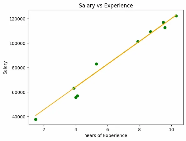
Visualization of Results

Elastic Net Regression effectively balances feature selection and model stability by combining Lasso and Ridge regularization. It’s a practical choice for handling datasets with many or highly correlated features, leading to more reliable and interpretable results.