Kernel Density Estimation (original) (raw)

Last Updated : 21 Jun, 2025

Kernel Density Estimation (KDE) is a non-parametric method used to estimate the probability density function (PDF) of a random variable. Unlike histograms, which use discrete bins, KDE provides a smooth and continuous estimate of the underlying distribution, making it particularly useful when dealing with continuous data.

Given a set of independent and identically distributed (i.i.d.) samples \{x_1, x_2, \dots, x_n\} from an unknown distribution with density function f(x), the goal is to estimate f(x) using only the samples.

The kernel density estimator \hat{f}_h(x) at a point x is defined as:

\hat{f}_h(x) = \frac{1}{n h} \sum_{i=1}^{n} K\left(\frac{x - x_i}{h}\right)

Where:

n is the number of data points.
h > 0 is the bandwidth (smoothing parameter).
K(\cdot) is the kernel function, which integrates to 1.

Each data point contributes a small "bump'' to the estimate, centered at x_i, and scaled by the bandwidth h. The final estimate is the sum of these bumps.

Kernel Functions

The kernel K(u) is typically a symmetric, non-negative function that integrates to 1. Common kernels include:

Kernel type	Function
Gaussian kernel	K(u) = \frac{1}{\sqrt{2\pi}} e^{-u^2/2}
Epanechnikov kernel	K(u) = \frac{3}{4}(1 - u^2), \quad \|u	\leq 1
Uniform kernel	K(u) = \frac{1}{2}, \quad \|u	\leq 1
Triangular kernel	K(u) = (1 - \|u	), \quad

The choice of kernel has a relatively minor impact on the final estimate compared to the choice of bandwidth h.

Bandwidth Selection

The bandwidth parameter h determines the smoothness of the density estimate. It controls how much the individual data points contribute to the overall estimate.

A small bandwidth produces a spiky estimate that may overfit the data.
A large bandwidth smooths the estimate too much, potentially hiding important features.

Optimal Bandwidth Formula

A commonly used formula for bandwidth is the Silverman’s Rule of Thumb:

h = 1.06 \sigma n^{-\frac{1}{5}}

where:

σ is the standard deviation of the data.
n is the number of observations.

Multivariate KDE

For d-dimensional data \mathbf{x}_i \in \mathbb{R}^d, KDE generalizes to:

\hat{f}_H(\mathbf{x}) = \frac{1}{n} \sum_{i=1}^{n} \frac{1}{\sqrt{|H|}} K\left(H^{-1/2}(\mathbf{x} - \mathbf{x}_i)\right)

Where:

H is a d \times d symmetric positive-definite bandwidth matrix.
K is a multivariate kernel (often a multivariate Gaussian).

Bandwidth matrix H controls smoothing in different directions and correlations among dimensions.

**Implementation in Python

Here’s how KDE is implemented using scipy:

Python `

import numpy as np import matplotlib.pyplot as plt from scipy.stats import gaussian_kde

Sample data

data = np.random.normal(0, 1, size=1000)

Using scipy

kde = gaussian_kde(data) x = np.linspace(-5, 5, 1000) plt.plot(x, kde(x), label='KDE (Scipy)') plt.hist(data, bins=30, density=True, alpha=0.3, label='Histogram') plt.legend() plt.show()

**Output:

kde

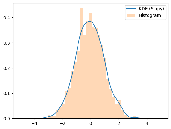
KDE plot using Scipy

**Variants and Improvements

**Adaptive KDE: Instead of using a global bandwidth, adaptive KDE varies bandwidth locally depending on the density of data points. Lower bandwidth is used in dense regions, and higher bandwidth in sparse areas.
**Fast KDE: Uses data structures like KD-trees or FFT-based convolutions to speed up computation. Libraries like statsmodels and sklearn offer optimized implementations.
**Boundary Correction: When estimating densities near the edge of the support (e.g. non-negative variables), KDE underestimates the density. Solutions include reflection and transformation techniques.

**Applications

**Data Visualization: KDE provides clearer plots for understanding the shape of data distributions, particularly in large datasets.
**Anomaly Detection: Points in low-density regions can be flagged as anomalies. KDE forms the basis for several unsupervised anomaly detection algorithms.
**Mode Estimation: KDE allows for identifying peaks in the distribution, which correspond to modes.
**Bayesian Inference: KDE is often used to approximate posterior distributions obtained via sampling (e.g. MCMC methods).
**Image Processing: In image segmentation and denoising, KDE helps in estimating the intensity distribution of pixels.

**Limitations and Challenges

**Curse of Dimensionality: KDE performs poorly in high-dimensional spaces. As dimensions increase, data sparsity grows, and KDE requires exponentially more samples for a reliable estimate.
**Computational Complexity: Evaluating the density at m points takes O(nm) time. This can be prohibitive for large datasets.
**Bandwidth Selection: Choosing an optimal bandwidth is difficult and often problem-specific. Poor choices lead to under- or over-smoothing.