Leveraging SHAP Values for Model Insights and Enhanced Performance (original) (raw)

Last Updated : 23 Jul, 2025

Machine learning models are often perceived as "black boxes" due to their complexity and lack of transparency. This opacity can be a significant barrier when it comes to understanding and trusting model predictions, especially in critical applications such as healthcare, finance, and legal systems. SHAP (SHapley Additive exPlanations) values offer a powerful solution to this problem by providing a clear and consistent method to interpret model predictions. In this article, we will delve into the technical aspects of SHAP values, their theoretical foundation, and practical implementation.

Table of Content

• What are SHAP Values?
  • Properties of SHAP Values
  • How SHAP Values Work?
  • Calculating SHAP Values
• Interpreting SHAP Values: A Practical Example
• Visualizing SHAP Values
• Practical Implementation with Python : Interpreting SHAP values
• Advantages and Disadvantages of Shap Values
  • Advantages of SHAP Values
  • Limitations of SHAP Values
• Applications of SHAP Values

What are SHAP Values?

SHAP values are a method based on cooperative game theory that provides explanations for individual predictions made by machine learning models. They quantify the contribution of each feature to the prediction, offering both global and local interpretability. SHAP values decompose a prediction into the contributions of each feature, ensuring that the sum of these contributions equals the difference between the actual prediction and the average prediction. This decomposition helps in understanding the influence of each feature on the model's output.

The concept of SHAP values is derived from Shapley values in cooperative game theory. In a game, the Shapley value represents the fair distribution of payoffs among players based on their contributions. Similarly, SHAP values distribute the "payoff" (model prediction) among features based on their contributions.

In this context, a "game" refers to the prediction task, and the "players" are the features of the model. SHAP values quantify the contribution of each feature to a specific prediction by considering all possible combinations of features. This approach provides a fair distribution of credit among the features, ensuring that the explanation is consistent and locally accurate.

Properties of SHAP Values

SHAP values possess several desirable properties that make them suitable for model interpretability:

• **Additivity: The sum of SHAP values for all features equals the difference between the model's prediction and the baseline (average) prediction.
• **Local Accuracy: SHAP values provide an accurate explanation for individual predictions.
• **Consistency: If a model changes such that a feature's contribution increases, its SHAP value will not decrease.
• **Missingness: Features that are not present in the model have a SHAP value of zero.

**How SHAP Values Work?

1. **Baseline Prediction: SHAP analysis starts by establishing a baseline prediction, which is usually the average prediction of the model across the entire dataset.
2. **Feature Permutations: Each feature is systematically removed from the model, and the impact on the prediction is measured. This process is repeated for all possible combinations of features.
3. **Shapley Value Calculation: By analyzing the changes in predictions resulting from these permutations, SHAP values are calculated for each feature. The Shapley value represents the average marginal contribution of a feature across all possible coalitions.
4. **Prediction Explanation: SHAP values are then used to explain individual predictions. Each feature's SHAP value indicates how much it pushed the prediction away from the baseline. Positive values imply the feature increased the prediction, while negative values imply it decreased it.

Calculating SHAP Values

Calculating SHAP values involves evaluating the contribution of each feature by considering all possible combinations of features. This can be computationally expensive, especially for models with many features. However, several approximation methods have been developed to make this feasible.

• **Exact SHAP Values: For small models, exact SHAP values can be computed by evaluating all possible feature combinations. This involves calculating the marginal contribution of each feature for every possible subset of features.
• **Approximation Methods: For larger models, approximation methods such as Kernel SHAP and Tree SHAP are used. Kernel SHAP is a model-agnostic method that approximates SHAP values using a weighted linear regression. Tree SHAP is a faster method specifically designed for tree-based models.

**Interpreting SHAP Values: A Practical Example

Let's consider a credit risk model. The features might include income, credit history, debt-to-income ratio, and employment status. SHAP values for a specific prediction might look like this:

• Income: +0.3
• Credit History: +0.5
• Debt-to-Income Ratio: -0.2
• Employment Status: +0.1

This indicates that a high income and good credit history increased the predicted probability of repayment. A high debt-to-income ratio slightly lowered it, while employment status had a minor positive influence.

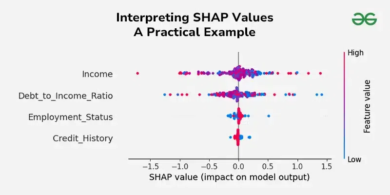
Interpreting SHAP Values

Visualizing SHAP Values

Visualization is a crucial aspect of interpreting SHAP values. The SHAP library provides several plots to help understand the contributions of features:

**1. Summary Plot

The summary plot shows the distribution of SHAP values for each feature across all predictions. It provides a global view of feature importance and the direction of their impact.

shap.summary_plot(shap_values, X_test)

**2. Dependence Plot

The dependence plot shows the relationship between a feature's value and its SHAP value, highlighting interactions with other features.

shap.dependence_plot("feature_name", shap_values, X_test)

**3. Force Plot

The force plot visualizes the SHAP values for a single prediction, showing how each feature contributes to the final prediction.

shap.force_plot(explainer.expected_value, shap_values[0], X_test.iloc[0])

Practical Implementation with Python : Interpreting SHAP values

Let's walk through a practical example of using SHAP values to explain a machine learning model in Python.

**Step 1: Install required Libraries

pip install shap scikit-learn

**Step 2: Load the required Libraries

Python `

import shap import pandas as pd from sklearn.datasets import fetch_california_housing from sklearn.ensemble import RandomForestRegressor from sklearn.model_selection import train_test_split

`

**Step 3: Load and Prepare the Dataset

Load the California housing(pre-built) dataset and prepare the dataset for model training.

Python `

Load the California housing dataset

housing = fetch_california_housing() X = pd.DataFrame(housing.data, columns=housing.feature_names) y = housing.target

Split the data into training and testing sets

X_train, X_test, y_train, y_test = train_test_split(X, y, test_size=0.2, random_state=42)

`

**Step 4: Train the Machine Learning Model

Now train a RandomForestRegressor model on the generated training data.

Python `

Train a Random Forest model

model = RandomForestRegressor(n_estimators=100, random_state=42) model.fit(X_train, y_train)

`

**Step 5: Calculate SHAP Values

Now we create a SHAP explainer based on the trained model and calculate SHAP values for the test set, with the additivity check disabled to avoid the discrepancy error.

Python `

Create a SHAP explainer

explainer = shap.Explainer(model, X_train)

Calculate SHAP values for the test set

shap_values = explainer(X_test)

`

**Step 6: Interpret SHAP Values

**1. Summary Plot:

• Displays the overall importance of each feature in the model.
• We can see the features at the top are the most important.
• Each colors indicate the feature value such as - red means high, blue means low.
• The horizontal spread of the datapoints shows how much the feature impacts the model's prediction. Python `

Summary plot

shap.summary_plot(shap_values, X_test)

`

**Output:

Summary Plot

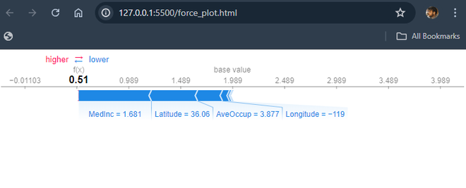
**2. Force Plot:

• It shows how each feature contributes to a single prediction.
• The starting point (expected value of the model).
• Features pushing the prediction higher are in red, while those pushing it lower are in blue.
• The final prediction is the sum of the base value and all feature contributions. Python `

Force plot for a single prediction

shap.initjs() shap.force_plot(explainer.expected_value, shap_values[0], X_test.iloc[0])

`

**Output:

Force Plot

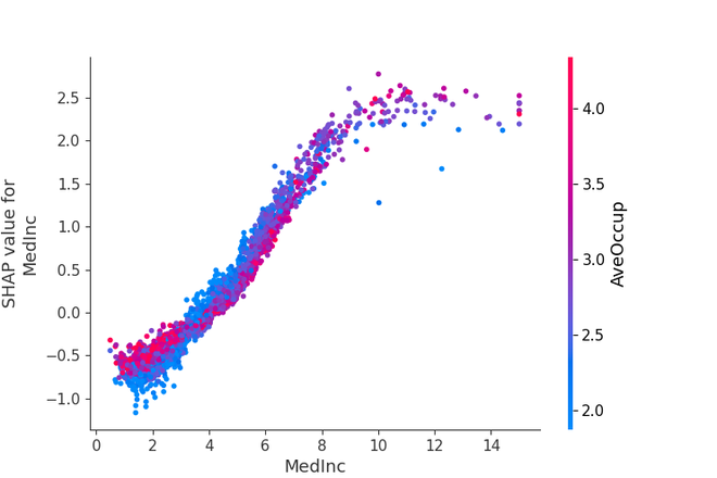
**3. Dependence Plot

• It shows the relationship between a specific feature and the SHAP values.
• Highlights how changes in the feature value impact the prediction.
• Secondary color coding shows interactions with another feature.
• Helps to see if the feature has a linear or non-linear effect on predictions. Python `

Dependence plot for a specific feature

shap.dependence_plot("MedInc", shap_values.values, X_test)

`

**Output:

Force Plot

Advantages and Disadvantages of Shap Values

**Advantages of SHAP Values

• **Model Agnostic: SHAP values can be applied to any ML model, regardless of its complexity or architecture.
• **Local Accuracy: SHAP values provide explanations for individual predictions, offering insight into how the model behaves in specific cases.
• **Global Interpretability: By aggregating SHAP values across the entire dataset, you can gain a comprehensive understanding of feature importance and interactions.
• **Contrasting Explanations: SHAP values allow you to compare the contributions of different features for different predictions, facilitating a deeper understanding of the model's decision boundaries.

Limitations of SHAP Values

• Calculating SHAP values can take a lot of time for big datasets and models that are very complicated.
• Understanding SHAP values needs knowledge about machine learning, which might not be easy for everyone.
• SHAP values are specific to the model they're calculated from and might not work as well with other types of models.
• While SHAP values give us some understanding, they might not completely explain how different parts of very complicated models work together.
• The results we get from SHAP values depend a lot on how good our data is. If the data is noisy or biased, the explanations we get might not be right.

**Applications of SHAP Values

• **Debugging Models: Identify and rectify biases or erroneous behavior by analyzing feature contributions.
• **Improving Model Performance: Gain insights into which features are most impactful and optimize the model accordingly.
• **Building Trust: Provide transparent explanations of predictions to stakeholders, regulators, and end-users.
• **Regulatory Compliance: Fulfill requirements for explainable AI in regulated industries like finance and healthcare.
• **Scientific Discovery: Uncover relationships and interactions between features that might not be apparent through other analysis methods.

Conclusion

SHAP (SHapley Additive exPlanations) values are a valuable tool for the machine learning models. It help us to see how each feature affects predictions, making models more perfect. By understanding the model behavior, we make decisions based on model insights. Except some challenges SHAP values greatly enhance our ability to check how machine learning effectively in real-world scenarios, gives more reliable and insightful results.