Implementing Linear Regression From Scratch using Python (original) (raw)

Last Updated : 5 Jun, 2026

Linear Regression is a supervised machine learning algorithm used to predict continuous values by modelling the relationship between input features and output using a best-fit straight line.

Predicts continuous outputs such as prices, scores, or sales values.
Learns the relationship between independent variables and the dependent variable from training data.

types_of_linear_regression

Types

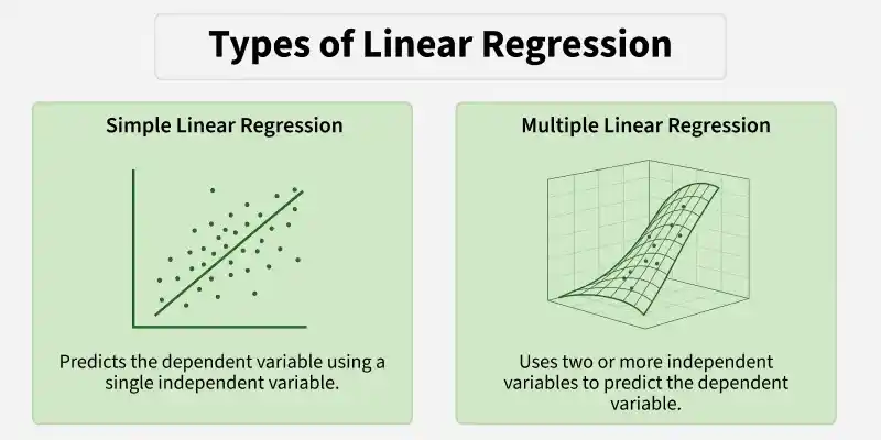
Linear Regression is mainly of two types:

1. Simple Linear Regression

Simple Linear Regression is a supervised learning algorithm used to predict a continuous target variable using a single input feature. It assumes a linear relationship between the input and output and represents it using a straight line.

**Step 1: Import Libraries

Import the required libraries NumPy for numerical operations and Matplotlib for visualization.

R `

import numpy as np import matplotlib.pyplot as plt

**Step 2: Implement Simple Linear Regression Class

Define a SimpleLinearRegression class to model the relationship between a single input feature and a target variable using a linear equation.

**__init__ method: Initializes slope, intercept, and R² attributes.
**fit method: Adds bias term, computes slope and intercept using the Normal Equation, and evaluates R² score.
**predict method: Adds bias to the input X and calculates predicted values using the learned coefficients. Python `

class SimpleLinearRegression: def init(self): self.coefficient_ = None self.intercept_ = None self.r2score_ = None

def fit(self, X, y):
    n = len(X)
    X_b = np.c_[np.ones((n,1)), X]  

    self.coefficients_ = np.linalg.inv(X_b.T.dot(X_b)).dot(X_b.T).dot(y)
    self.intercept_ = self.coefficients_[0]
    y_pred = X_b.dot(self.coefficients_)
    # R²
    self.r2score_ = 1 - (np.sum((y - y_pred)**2) / np.sum((y - np.mean(y))**2))
    self.y_pred_ = y_pred
    
def predict(self, X):
    X_b = np.c_[np.ones((len(X),1)), X]
    return X_b.dot(self.coefficients_)

**Step 3: Fit the Model and Visualize Results

Fit the model to training data and compute coefficients along with R² score and and plot the data points along with the best-fit regression line.

Python `

X_simple = np.array([1,2,3,4,5,6,7,8,9,10]).reshape(-1,1) y_simple = np.array([2,4,5,4,5,7,8,9,10,12])

slr = SimpleLinearRegression() slr.fit(X_simple, y_simple)

print(f"Simple LR Coefficients: {slr.coefficients_}") print(f"R² Score: {slr.r2score_:.2f}")

plt.scatter(X_simple, y_simple, color='blue', label='Data') plt.plot(X_simple, slr.y_pred_, color='red', label='Regression Line') plt.title("Simple Linear Regression") plt.xlabel("X") plt.ylabel("y") plt.legend() plt.show()

**Output:

Screenshot-2026-03-12-171911

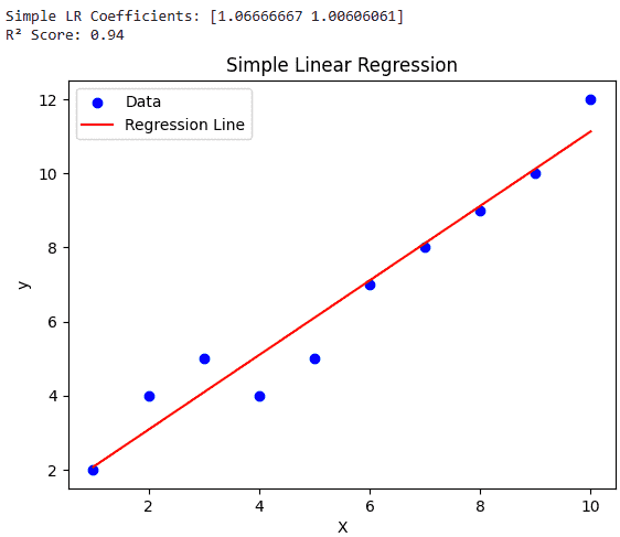
Simple Linear Regression

2. Multiple Linear Regression

Multiple Linear Regression is used to predict a continuous target variable based on two or more input features, assuming a linear relationship between the inputs and the output.

**Step 1: Import Libraries

Import NumPy for numerical operations, Matplotlib for plotting and mpl_toolkits.mplot3d to create 3D visualizations.

Python `

import numpy as np import matplotlib.pyplot as plt from mpl_toolkits.mplot3d import Axes3D

**Step 2: Implement Multiple Linear Regression Class

Here we implement a Multiple Linear Regression class to model the relationship between multiple input features and a continuous target variable using a linear equation.

__init__ method: Initializes coefficients (slopes), intercept (bias), and R² score for model evaluation.
fit method: Adds bias term, computes coefficients using the Normal Equation, predicts outputs, and calculates R² score.
predict method: Adds bias to input data and generates predictions using learned coefficients. Python `

class MultipleLinearRegression: def init(self): self.coefficients_ = None self.intercept_ = None
self.r2score_ = None

def fit(self, X, y):
    n = X.shape[0]
    X_b = np.c_[np.ones((n,1)), X]  
    self.coefficients_ = np.linalg.inv(X_b.T.dot(X_b)).dot(X_b.T).dot(y)
    self.intercept_ = self.coefficients_[0]
    y_pred = X_b.dot(self.coefficients_)
    self.r2score_ = 1 - (np.sum((y - y_pred)**2)/np.sum((y - np.mean(y))**2))
    self.y_pred_ = y_pred
    
def predict(self, X):
    X_b = np.c_[np.ones((X.shape[0],1)), X]  
    return X_b.dot(self.coefficients_)

**Step 3: Generate Sample Dataset

We create a small dataset with two input features and a target variable, adding noise to simulate real-world data.

Python `

np.random.seed(0) X1 = np.random.randint(1, 11, 15) X2 = np.random.randint(1, 11, 15) X_multi = np.column_stack((X1, X2)) y_multi = 1 + 2X1 + 3X2 + np.random.randn(15)*2

**Step 4: Fit the Model and Visualize

We train the Multiple Linear Regression model on the dataset, print coefficients and R² score, and visualize the regression plane in 3D.

Python `

mlr = MultipleLinearRegression() mlr.fit(X_multi, y_multi) print(f"Multiple LR Coefficients: {mlr.coefficients_}") print(f"R² Score: {mlr.r2score_:.2f}")

fig = plt.figure(figsize=(10,7)) ax = fig.add_subplot(111, projection='3d')

ax.scatter(X_multi[:,0], X_multi[:,1], y_multi, color='blue', label='Data')

x1_surf, x2_surf = np.meshgrid( np.linspace(X_multi[:,0].min(), X_multi[:,0].max(), 10), np.linspace(X_multi[:,1].min(), X_multi[:,1].max(), 10) )

pred_surf = mlr.predict(np.c_[x1_surf.ravel(), x2_surf.ravel()]).reshape(x1_surf.shape)

ax.plot_surface(x1_surf, x2_surf, pred_surf, color='red', alpha=0.5, rstride=1, cstride=1)

ax.set_xlabel('X1') ax.set_ylabel('X2') ax.set_zlabel('y') ax.set_title("Multiple Linear Regression with Regression Plane") ax.legend() plt.show()

**Output:

Screenshot-2026-03-12-173056

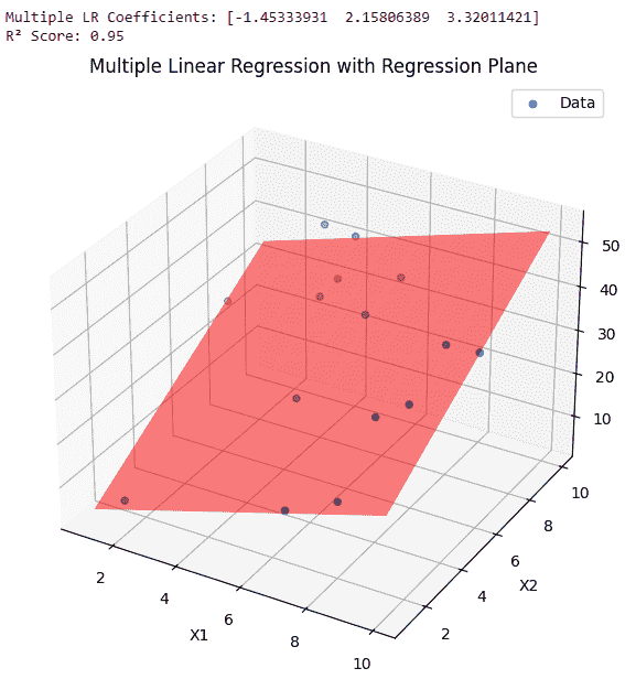
Multiple linear regression

Download code from here.