Locally Linear Embedding in Machine Learning (original) (raw)
Last Updated : 24 Oct, 2025
Locally Linear Embedding (LLE) is a non-linear dimensionality reduction technique used in machine learning to uncover meaningful structures in high-dimensional data. Unlike linear methods such as PCA, LLE preserves the local relationships among data points making it effective for visualizing and analyzing complex datasets without losing the important shape or structure of the data.
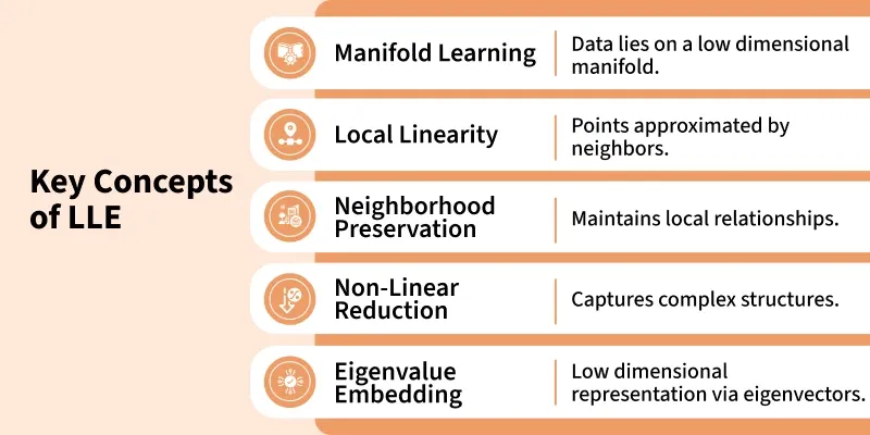
Concepts
Importance in Dimensionality Reduction
LLE is important in dimensionality reduction because:
- **Preserves Local Structures: Maintains relationships between neighbouring points.
- **Captures Non Linear Patterns: Models complex manifolds beyond linear methods.
- **Reduces Dimensionality: Simplifies high-dimensional data for analysis.
- **Improves Visualization: Projects data into 2D or 3D for exploration.
- **Reveals Hidden Structures: Uncovers latent patterns not visible in the original space.
- **Enhances Feature Extraction: Identifies intrinsic features for downstream tasks.
- **Facilitates Similarity Analysis: Preserves neighbourhoods for clustering or similarity measures.
- **Supports Noise Reduction: Filters out irrelevant variations in data.
Consider a Swiss roll dataset a 3D shape that looks like a rolled up sheet. Even though it’s curved and complex LLE can “unroll” it into a flat 2D shape while keeping the original structure and relationships between points.
**Working
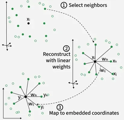
The LLE algorithm can be broken down into several steps:
Workflow
**1. Neighborhood Selection:
- For each data point in the high dimensional space, it identifies its k-nearest neighbors.
- This step is crucial because it assumes each point can be approximated by a linear combination of its neighbors capturing local structure.
**2. Weight Matrix Construction:
- It computes weights for each point to represent it as a linear combination of its neighbors.
- The weights are chosen to minimize reconstruction error often using linear regression.
- All weights together form a weight matrix that encodes local relationships in the dataset.
**3. Global Structure Preservation:
- Using the weight matrix, It finds a lower dimensional embedding that best preserves these local linear relationships.
- This is done by minimizing a cost function that measures how well each point can be reconstructed from its neighbors in the reduced space.
**4. Output Embedding:
- The result is a low dimensional representation of the data that captures the essential structure while preserving neighborhood relationships.
- This embedding can be used for visualization, clustering or further analysis.
Mathematical Implementation of LLE Algorithm
Here’s a basic overview of how it works mathematically:
**1. Neighborhood Selection:
- For each data point x_i \in {R}^D, identify its k-nearest neighbors x_j.
- Let the neighbors of x_ibe N(i).
**2. Compute Reconstruction Weights:
- Represent x_ias a linear combination of its neighbors:
x_i \approx \sum_{j \in N(i)} w_{ij} x_j
- Minimize the reconstruction error to find weights w_{ij}:
\epsilon(W) = \sum_i \left\| x_i - \sum_{j \in N(i)} w_{ij} x_j \right\|^2
- Constraint: \sum_{j \in N(i)} w_{ij} = 1.
- Usually solved using linear regression.
**3. Compute Low Dimensional Embedding:
- Find low dimensional vectors y_i \in \mathbb{R}^d \quad (d \ll D)that preserve the weights:
\Phi(Y) = \sum_i \left\| y_i - \sum_{j \in N(i)} w_{ij} y_j \right\|^2
- Center: \sum_i y_i = 0
- Scale: \frac{1}{N} \sum_i y_i y_i^T = I
- Solve the eigenvalue problem: M Y = \lambda Y, \quad M = (I - W)^\top (I - W)
- Select the bottom d+1 eigenvectors, discard the smallest eigenvector corresponding to eigenvalue 0.
**4. Output: The resulting low dimensional coordinates Y preserve the local linear structure of the original high dimensional data.
Parameters in LLE Algorithm
LLE has a few parameters that influence its behavior:
**1. n_neighbors: Number of nearest neighbors to use for reconstructing each data point. A critical parameter that affects the quality of the embedding.
**2. n_components: The target number of dimensions for the reduced space like 2 or 3 for visualization.
**3. reg (Regularization): Small regularization term added to the weights to handle cases of bad conditioned matrices improving numerical stability.
**4. eigen_solver: Algorithm used to solve the eigenvalue problem. Choice depends on dataset size and efficiency needs.
**5. method: Specifies the LLE variant:
- **standard: Basic LLE.
- **modified: Improves robustness to noise.
- **hessian: Hessian Eigenmaps captures curvature.
- **ltsa: Local Tangent Space Alignment which are better for manifolds.
**6. max_iter and tol: Maximum iterations and tolerance for convergence in the eigenvalue solver.
**7. random_state: Controls randomness in certain solvers for reproducibility.
Implementation
**1. Importing Libraries
Importing libraries like Numpy, Matplotlib and Scikit-Learn modules.
Python `
import numpy as np import matplotlib.pyplot as plt from sklearn.datasets import make_swiss_roll from sklearn.manifold import LocallyLinearEmbedding
`
**2. Generate a Synthetic Dataset (Swiss Roll)
Generating a synthetic dataset resembling a Swiss Roll using the make_swiss_roll function from scikit-learn.
- **n_samples: Specifing the number of data points to generate.
- **n_neighbors: Defining the number of neighbors used in the LLE algorithm. Python `
n_samples = 1000 n_neighbors = 10 X, _ = make_swiss_roll(n_samples=n_samples)
`
**3. Apply Locally Linear Embedding (LLE)
- An instance of the LLE algorithm is created with LocallyLinearEmbedding.
- The n_neighbors parameter determines the number of neighbors to consider during the embedding process.
- The LLE algorithm is then fitted to the original data X using the fit_transform method reducing the dataset to two dimensions (n_components=2). Python `
lle = LocallyLinearEmbedding(n_neighbors=n_neighbors, n_components=2) X_reduced = lle.fit_transform(X)
`
**4. Visualize the Original and Reduced Data
- After reducing dimensions with LLE we plot the original high dimensional data and the new lower dimensional data.
- This helps us see if important patterns are preserved and easier to understand. Python `
plt.figure(figsize=(12, 6))
plt.subplot(121) plt.scatter(X[:, 0], X[:, 1], c=X[:, 2], cmap=plt.cm.Spectral) plt.title("Original Data") plt.xlabel("Feature 1") plt.ylabel("Feature 2")
plt.subplot(122) plt.scatter(X_reduced[:, 0], X_reduced[:, 1], c=X[:, 2], cmap=plt.cm.Spectral) plt.title("Reduced Data (LLE)") plt.xlabel("Component 1") plt.ylabel("Component 2")
plt.tight_layout() plt.show()
`
**Output:

Locally Linear Embedding
- The second subplot shows the LLE-reduced data (X_reduced), colored by the third original feature (X[:, 2]).
- plt.tight_layout() ensures proper spacing between subplots.
Comparison with Other Techniques
Comparison table of LLE, PCA, Isomap and t-SNE:
| Feature | PCA | LLE | Isomap | t-SNE |
|---|---|---|---|---|
| Type | Linear | Non Linear | Non Linear | Non Linear |
| Goal | Maximize variance | Preserve local structure | Preserve global distances | Preserve local similarities |
| Global Structure | Yes | No | Yes | No |
| Local Structure | Limited | Yes | Yes | Yes |
| Computational Cost | Low | Moderate | Moderate-High | High |
| Best Use | Linear datasets | Non Linear manifolds | Non Linear with global structure | High dimensional visualization |
Applications
Here are some of the applications of LLE:
- **Image Processing: Used in face recognition, handwriting analysis and other image related tasks by capturing non linear patterns and reducing dimensions for easier processing.
- **Speech and Audio Analysis: Helps in modeling complex patterns in speech or audio signals preserving local structures for feature extraction and classification.
- **Data Visualization: Projects high dimensional data into 2D or 3D for exploration and pattern recognition making it easier to identify clusters or structures.
- **Manifold Learning in Biology: Used to study gene expression or biological data where samples lie on a non linear manifold preserving neighborhood relationships.
- **Anomaly Detection: Assists in identifying unusual patterns or clusters in datasets by reducing dimensions while maintaining local relationships.
Advantages
Some of the advantages of LLE are:
- **Preservation of Local Structures: Maintains the local neighborhood relationships in the data preserving distances between nearby points and capturing the natural shape of the dataset.
- **Handling Non Linearity: Unlike PCA which only captures linear patterns, LLE can model complex non-linear structures making it effective for datasets lying on curved manifolds.
- **Dimensionality Reduction: Reduces high dimensional data into fewer dimensions while keeping important properties intact making it easier to visualize and analyze.
- **Good for Visualization: Projects data into 2D or 3D spaces without losing much structure, useful for exploring high dimensional datasets.
- **Unsupervised Learning: Does not require labels so it works well for exploratory data analysis in various domains like images, speech or genetics.
Disadvantages
Some of the disadvantages of LLE are:
- **Sensitive to Parameters: The choice of the number of neighbors (
k) is crucial, a poor selection can distort the embedding and reduce accuracy. - **No Out-of-Sample Mapping: It doesn't provide a direct transformation for new, unseen data, the algorithm must be re-run for additional samples.
- **Sensitive to Noise and Outliers: Unusual or noisy data points can distort local neighborhoods leading to poor embeddings.
- **Loss of Global Structure: Focuses on preserving local relationships but may ignore global data patterns and distances.
- **Curse of Dimensionality: In very high dimensional spaces, more neighbors are needed to capture local structures which increases computational costs.