Machine Learning Interview Questions and Answers (original) (raw)
Last Updated : 6 Oct, 2025
Machine Learning concepts form the foundation of how models are built, trained and evaluated. From understanding supervised and unsupervised learning, to working with algorithms like regression, decision trees and neural networks, every concept plays a role in solving real-world problems. In interviews, questions are often asked around these core ideas, testing both theoretical knowledge and practical application.
**1. What do you understand by Machine Learning (ML) and how does it differ from artificial intelligence (AI) and Data Science?
Machine Learning (ML) is a branch of Artificial Intelligence that deals with building algorithms capable of learning from data. Instead of being explicitly programmed with fixed rules, these algorithms identify patterns in data and use them to make predictions or decisions that improve with experience.
| Aspect | Artificial Intelligence (AI) | Machine Learning (ML) | Data Science |
|---|---|---|---|
| **Definition | Broad field aiming to build systems that mimic human intelligence | Subset of AI that learns patterns from data for prediction or decision-making | Field focused on extracting insights and knowledge from data |
| **Scope | Reasoning, problem-solving, planning, natural language, robotics | Algorithms for classification, regression, clustering, etc. | Data collection, cleaning, analysis, visualization, ML and reporting |
| **Techniques Used | Expert systems, NLP, robotics, ML, deep learning | Regression, decision trees, neural networks, clustering | Statistics, ML, data visualization, domain knowledge |
| **Example | Chatbots, self-driving cars, expert systems | Spam detection, recommendation systems, fraud detection | Analyzing sales trends, customer segmentation, forecasting |
**2. What is overfitting in machine learning and how can it be avoided?
**1. Overfitting: It occurs when a model not only learns the true patterns in the training data but also memorizes the noise or random fluctuations. This results in high accuracy on training data but poor performance on unseen/test data.
**Ways to Avoid Overfitting:
- **Early Stopping: Stop training when validation accuracy stops improving, even if training accuracy is still increasing.
- **Regularization: Apply techniques like L1 (Lasso) or L2 (Ridge) regularization which add penalties to large weights to reduce model complexity.
- **Cross-Validation: Use k-fold cross-validation to ensure the model generalizes well.
- **Dropout (for Neural Networks): Randomly drop neurons during training to prevent over-reliance on specific nodes.
- **Simpler Models: Avoid overly complex models when simpler ones can explain the data well.
**2. Underfitting: It occurs when a model is too simple to capture the underlying patterns in the data. This leads to poor accuracy on both training and test data.
**Ways to Avoid Underfitting:
- **Use a More Complex Model: Choose models with higher complexity to learn pattern like decision trees, neural networks, etc.
- **Add Relevant Features: Include meaningful features that better represent the data.
- **Reduce Regularization: Too much regularization can restrict the model’s ability to learn.
- **Train Longer: Allow the model more epochs or iterations to properly learn patterns.
3. What is Regularization?
Regularization is a technique used to reduce model complexity and prevent overfitting. It works by adding a penalty term to the loss function to discourage the model from assigning too much importance (large weights) to specific features. This helps the model generalize better on unseen data.
**Ways to Apply Regularization:
- **L1 Regularization (Lasso): Adds the absolute value of weights as a penalty which can shrink some weights to zero and perform feature selection.
- **L2 Regularization (Ridge): Adds the squared value of weights as a penalty which reduces large weights but doesn’t eliminate them.
- **Elastic Net: Combines both L1 and L2 penalties to balance feature selection and weight reduction.
- **Dropout (for Neural Networks): Randomly drops neurons during training to avoid over-reliance on specific nodes.
4. Explain Lasso and Ridge Regularization. How do they help in Elastic Net Regularization?
**1. Lasso Regularization (L1): Lasso adds a penalty equal to the absolute value of the model’s weights to the loss function. It can shrink some weights to exactly zero, performing feature selection.
**Formula:
\text{Lasso Loss} = \text{MSE} + \lambda \sum_{i=1}^{n} |w_i|
Where:
- MSE = Mean Squared Error
- w_i = model weights
- \lambda = regularization strength
**2. Ridge Regularization (L2): It adds a penalty equal to the square of the model’s weights to the loss function. It reduces large weights but does not set them to zero, helping generalization.
**Formula:
\text{Ridge Loss} = \text{MSE} + \lambda \sum_{i=1}^{n} w_i^2
Where:
- MSE = Mean Squared Error
- w_i = model weights
- \lambda = regularization strength
**Key Differences:
- **Lasso (L1): Can set weights to zero → feature selection. Use it when we have many irrelevant features.
- **Ridge (L2): Reduces weights but keeps all features → no feature elimination. Use when all features are useful but want to avoid overfitting.
**3. Elastic Net Regularization: Elastic Net combines both L1 (Lasso) and L2 (Ridge) penalties, balancing feature selection and weight reduction. It is especially useful when features are correlated, as it avoids Lasso’s limitation of picking only one feature from a group.
5. What are different Model Evaluation Techniques in Machine Learning?
Model evaluation techniques are used to assess how well a machine learning model performs on unseen data. Choosing the right technique depends on the type of problem like classification, regression, etc and type of dataset we have.
- **Train-Test Split: Divide data into training and testing sets like 70:30 or 80:20 to evaluate model performance on unseen data. Here 70% data will be used for training and 30% will be used to test accuracy of model.
- **Cross-Validation: Split data into k folds, train on k-1 folds, validate on the remaining fold and average the results to reduce bias.
- **Confusion Matrix (for Classification): Counts True Positives, True Negatives, False Positives and False Negatives.
- **Accuracy: Proportion of correct predictions over total predictions.
- **Precision: Here correct positive predictions are divided by Total predicted positives.
- **Recall (Sensitivity): Here correct positive predictions are divided by Total actual positives.
- **F1-Score: Harmonic mean of precision and recall. It balances precision and recall.
- **ROC Curve & AUC: Measures model’s ability to distinguish between classes. Here AUC is area under the ROC curve.
- **Loss Functions (for Regression/Classification): Quantifies prediction error to optimize model. It can include: Mean Absolute Error (MAE), Mean Squared Error (MSE), Root Mean Squared Error (RMSE), etc.
6. Explain Confusion Matrix.
A confusion matrix is a table used to evaluate the performance of a classification model. It compares the predicted labels with the actual labels, telling how well the model is performing and what types of errors it makes.

Confusion Matrix
Here:
- **True Positives (TP): Correctly predicted positive cases.
- **True Negatives (TN): Correctly predicted negative cases.
- **False Positives (FP): Negative cases incorrectly predicted as positive.
- **False Negatives (FN): Positive cases incorrectly predicted as negative.
It is used in metrics like Accuracy, Precision, Recall and F1-Score.
7. What is the difference between precision and recall? How F1 combines both?
**1. Precision: It is the ratio between the true positives(TP) and all the positive examples (TP+FP) predicted by the model. In other words, precision measures how many of the predicted positive examples are actually true positives. It is a measure of the model's ability to avoid false positives and make accurate positive predictions.
\text{Precision}=\frac{TP}{TP\; +\; FP}
Example: In spam detection, high precision means most emails marked as spam are truly spam.
**2. Recall: It calculate the ratio of true positives (TP) and the total number of examples (TP+FN) that actually fall in the positive class. Recall measures how many of the actual positive examples are correctly identified by the model. It is a measure of the model's ability to avoid false negatives and identify all positive examples correctly.
\text{Recall}=\frac{TP}{TP\; +\; FN}
Example: In disease detection, high recall means most sick patients are correctly identified.
**Key Difference:
- Precision is about being exact (avoiding false positives).
- Recall is about being comprehensive (avoiding false negatives).
**3. F1-Score (Balance of Both): Used when both precision and recall matter.
F1 = 2 \times \frac{\text{Precision} \times \text{Recall}}{\text{Precision + Recall}}
8. Different Loss Functions in Machine Learning
Loss functions measure the error between the model’s predicted output and the actual target value. They guide the optimization process during training. Some of them are:
**1. Mean Squared Error (MSE): Used in regression problem. It penalizes larger errors more heavily by squaring them.
MSE = \frac{1}{n}\sum_{i=1}^{n}(y_i - \hat{y}_i)^2
**2. Mean Absolute Error (MAE): Used in regression as it takes absolute differences between predicted and actual values. It is less sensitive to outliers than MSE.
MAE = \frac{1}{n}\sum_{i=1}^{n}\lvert y_i - \hat{y}_i \rvert
**3. Huber Loss: It combines MSE and MAE making it less sensitive to outliers than MSE.
**4. Cross-Entropy Loss (Log Loss): Used in classification problem. It measures the difference between predicted probability distribution and actual labels.
CE = -\frac{1}{n} \sum_{i=1}^{n}\big[y_i \log(\hat{y}_i) + (1-y_i)\log(1-\hat{y}_i)\big]
**5. Hinge Loss: Used for classification with SVMs. It encourages maximum margin between classes.
**6. KL Divergence: Measures how one probability distribution differs from another hence used in probabilistic models.
**7. Exponential Loss: Used in boosting methods like AdaBoost; penalizes misclassified points more strongly.
**8.R-squared (R²): Used in regression and measures how well the model explains variance in the target variable.
R^2 = 1 - \frac{\sum_{i=1}^{n} (y_i - \hat{y}_i)^2}{\sum_{i=1}^{n} (y_i - \bar{y})^2}
9. What is AUC–ROC Curve?
**ROC Curve (Receiver Operating Characteristic): The ROC curve is a graphical plot that shows the trade-off between True Positive Rate (TPR / Recall) and False Positive Rate (FPR) at different threshold values.
- **TPR (Recall): TPR = \frac{TP}{TP + FN}
- **FPR: FPR = \frac{FP}{FP + TN}
**AUC (Area Under the Curve): AUC is the area under the ROC curve. It represents the probability that a randomly chosen positive instance is ranked higher than a randomly chosen negative instance.
- AUC = 1 → Perfect classifier
- AUC = 0.5 → Random guessing
- AUC < 0.5 → Worse than random
ROC shows performance across thresholds. AUC summarizes overall model performance into a single number.
**Example: If a medical test has an AUC of 0.90, it means there’s a 90% chance that the model will rank a randomly chosen diseased patient higher than a healthy one.
**10. Is accuracy always a good metric for classification performance?
No, accuracy can be misleading, especially with imbalanced datasets. In such cases:
- Precision and Recall provide better insight into model performance.
- F1-score combines precision and recall as their harmonic mean, giving a balanced measure of model effectiveness, especially when the classes are imbalanced.
11. What is Cross-Validation?
Cross-validation is a model evaluation technique used to test how well a machine learning model generalizes to unseen data. Instead of training and testing on a single split, the dataset is divided into multiple subsets (called folds) and the model is trained and tested multiple times on different folds.
**How It Works:
- Split the dataset into k folds like 5 or 10.
- Train the model on (k-1) folds and test it on the remaining fold.
- Repeat this process k times so that every fold is used for testing once.
- Take the average of all results as the final performance score.
**Types of Cross-Validation:
- **k-Fold Cross-Validation: Dataset is divided into k equal fold and training/testing is repeated k times.
- **Stratified k-Fold: Similar to k-Fold but keeps class distribution balanced (useful in classification).
- **Leave-One-Out (LOO): Special case where k = number of samples and every single point acts as a test set once.
- **Hold-Out Method: Simple train/test split and is considered a basic form of validation.
12. Explain k-Fold Cross-Validation, Leave-One-Out (LOO) and Hold-Out Method.
**1. k-Fold Cross-Validation: The dataset is divided into k equal folds. The model is trained on (k-1) folds and tested on the remaining fold. This process is repeated k times, with each fold used once as the test set. The final score is the average of all k test results.
CV_{error} = \frac{1}{k} \sum_{i=1}^{k} error_i
**2. Leave-One-Out Cross-Validation (LOO): A special case of k-Fold where k = number of samples. Each observation is used once as the test set while the remaining data is used for training. It gives very accurate estimates but is computationally expensive for large datasets.
**3. Hold-Out Method: The simplest technique where the dataset is split into two parts: a training set and a testing set (e.g., 70% train, 30% test). The model is trained on the training set and evaluated on the test set. It is fast but may lead to biased results depending on the split.
13. Difference Between Regularization, Standardization and Normalization
**1. Regularization: A technique used to reduce overfitting by adding a penalty term to the model’s loss function, discouraging overly complex models. Examples are: L1 (Lasso), L2 (Ridge), Elastic Net.
Works on model parameters (weights).
**2. Standardization: A preprocessing step that rescales features so they have mean = 0 and standard deviation = 1
x' = \frac{x - \mu}{\sigma}
Useful for algorithms sensitive to feature scales like SVM, KNN, Logistic Regression, etc.
**3. Normalization: A preprocessing step that rescales feature values into a fixed range, usually [0, 1].
x' = \frac{x - x_{min}}{x_{max} - x_{min}}
Useful when features have very different scales or units.
| Aspect | Regularization | Standardization | Normalization |
|---|---|---|---|
| Purpose | Prevent overfitting | Rescale features (mean = 0, std = 1) | Rescale features to a range (e.g., [0,1]) |
| Works On | Model weights | Input features | Input features |
| Main Idea | Add penalty to loss function | Center and scale features | Shrink features into fixed range |
| Example Techniques | L1, L2, Elastic Net | Z-score scaling | Min-Max scaling |
| When to Use | High variance/overfitting | Algorithms needing Gaussian-like distribution | Features with different ranges/units |
14. What is Feature Engineering in Machine Learning?
Feature engineering is the process of creating, transforming or selecting relevant features from raw data to improve the performance of a machine learning model. Better features often lead to better model accuracy and generalization. It also reduces overfitting and make the model easier to interpret.
**Key Steps in Feature Engineering:
- **Feature Creation: Generate new features from existing data like extracting “year” or “month” from a date column.
- **Feature Transformation: Apply scaling, normalization or mathematical transformations (log, square root) to features.
- **Feature Encoding: Convert categorical variables into numerical form like one-hot encoding, label encoding.
- **Feature Selection: Identify and keep only the most relevant features using techniques like correlation analysis, mutual information or model-based importance scores.
Example:
- Raw data: Date of Birth → Feature engineered: Age
- Raw data: Text review → Feature engineered: Sentiment score
15. Difference between Feature Engineering and Feature Selection?
| Aspect | Feature Engineering | Feature Selection |
|---|---|---|
| **Definition | Process of creating, transforming or deriving new features from raw data to improve model performance. | Process of selecting the most relevant features from the existing dataset to reduce noise and improve model performance. |
| **Purpose | To enhance or create meaningful features that the model can learn from. | To remove irrelevant or redundant features and simplify the model. |
| **Process | Involves feature creation, transformation, encoding, scaling, etc. | Involves statistical tests, correlation analysis, mutual information or model-based importance scores. |
| **Output | New or transformed features added to the dataset. | Subset of the original features retained for modeling. |
| **Example | Extracting Age from Date of Birth or generating sentiment scores from text. | Selecting top 10 features with highest importance from 50 features using Random Forest. |
**16. Feature Selection Techniques in Machine Learning
Feature selection is the process of choosing the most relevant features from your dataset to improve model performance, reduce overfitting and simplify the model.
**1. Filter Methods: Filter methods evaluate each feature independently with target variable. Feature with high correlation with target variable are selected as it means this feature has some relation and can help us in making predictions. Here features are selected based on statistical measures without involving any machine learning model.
Examples:
- **Correlation Coefficient: Remove features highly correlated with others.
- **Chi-Square Test: For categorical features.
- **ANOVA F-Test: For numerical features.
**2. Wrapper Methods: It uses different combination of features and compute relation between these subset features and target variable and based on conclusion addition and removal of features are done. Stopping criteria for selecting the best subset are usually pre-defined by the person training the model such as when the performance of the model decreases or a specific number of features are achieved.
Examples:
- **Forward Selection: Start with no features and add one at a time.
- **Backward Elimination: Start with all features and remove one at a time.
- **Recursive Feature Elimination (RFE): Iteratively removes least important features using model weights.
**3. Embedded Methods: Embedded methods perform feature selection during the model training process allowing the model to select the most relevant features based on the training process dynamically.
Examples:
- **Lasso Regression (L1 regularization): Can shrink some feature coefficients to zero.
- **Decision Tree / Random Forest Feature Importance: Select features based on importance scores learned during training.
17. What is Dimensionality Reduction in Machine Learning?
Dimensionality reduction is the process of reducing the number of features (variables) in a dataset while retaining most of the important information. It helps in simplifying models, improving performance, reducing overfitting and speeding up computation. Feature selection and Engineering comes under this.
- Reduces computational cost for high-dimensional datasets.
- Helps visualize data in 2D or 3D space.
- Reduces overfitting by removing irrelevant or noisy features.
**Example: A dataset has 100 features. Using PCA, it can be reduced to 10 principal components that capture 95% of the variance.
18. What is Categorical Data and how to handle it?
Categorical data refers to features that represent discrete values or categories, rather than continuous numerical values. Examples include gender (Male, Female), color (Red, Blue, Green) or product type (Electronics, Clothing).
Types of Categorical Data:
- **Nominal: Categories with no inherent order. Example: Red, Blue, Green.
- **Ordinal: Categories with a meaningful order. Example: Low, Medium, High.
Machine learning models require numerical inputs, so categorical data needs to be handelled using encoding. Common techniques include:
**1. Label Encoding:
- Converts each category into a unique integer.
- Example:
Red=0, Blue=1, Green=2. - Suitable for ordinal data.
**2. One-Hot Encoding:
- Converts categories into binary vectors, creating a new column for each category.
- Example:
ColorwithRed, Blue, Greenbecomes three columns:[1,0,0], [0,1,0], [0,0,1]. - Suitable for nominal data.
**3. Binary Encoding:
- Converts categories into binary code, reducing dimensionality compared to one-hot encoding.
**4. Target / Mean Encoding:
- Replaces categories with mean of target variable for regression or probability of positive class in classification.
19. Difference between label encoding and one hot encoding?
| Aspect | Label Encoding | One-Hot Encoding |
|---|---|---|
| **Definition | Converts each category into a unique integer. | Converts categories into binary vectors with separate columns for each category. |
| **Use Case | Suitable for ordinal data (ordered categories). | Suitable for nominal data (unordered categories). |
| **Example | Color: Red=0, Blue=1, Green=2 | Color: Red → [1,0,0], Blue → [0,1,0], Green → [0,0,1] |
| **Model Interpretation | May introduce false ordinal relationship for nominal features. | Preserves categorical nature without implying order. |
| **Output Dimension | 1 column, integer values | N columns (N = number of categories) |
| **Pros | Simple, compact representation | Avoids false relationships between categories |
| **Cons | Can mislead models if data is nominal | Increases dimensionality for high-cardinality features |
20. What is Upsampling and Downsampling?
Upsampling and downsampling are techniques used to handle imbalanced datasets where the number of samples in different classes is unequal.
**1. Upsampling (Oversampling): Increases the number of samples in the minority class to balance the dataset.Techniques include:
- **Random Oversampling: Duplicate random samples from the minority class.
- **SMOTE (Synthetic Minority Over-sampling Technique): Generate synthetic samples by interpolating between existing minority samples.
**2. Downsampling (Undersampling): Reduces the number of samples in the majority class to balance the dataset. Techniques include:
- **Random Undersampling: Randomly remove samples from the majority class.
- **Cluster-Based Undersampling: Remove samples based on clustering to retain diversity.
**Example: We have a dataset of 1000 positive samples, 100 negative samples.
- Upsampling create 900 additional negative samples.
- Downsampling reduce positive samples to 100.
**21. Explain SMOTE method used to handle data imbalance
SMOTE (Synthetic Minority Over-sampling Technique) creates synthetic data points for minority classes using linear interpolation between existing samples.
- The model is trained on more diverse examples rather than duplicating existing points.
- It may introduce noise into the dataset, potentially affecting model performance if overused.
22. How to handle missing and duplicate values****?**
Missing values are common in real-world datasets and can affect model performance. Techniques to Handle Missing Values are:
**1. Remove Rows or Columns:
- Drop rows with missing values using
dropna()in pandas. - Drop columns if most values are missing.
**2. Imputation:
- **Mean/Median/Mode Imputation: Replace missing values with mean/median (for numerical) or mode (for categorical).
- **Forward/Backward Fill: Fill missing values using previous or next valid value in time series data.
- **Prediction-Based Imputation: Predict missing values using a model trained on other features.
**3. Flag Missing Values:
- Create a new binary column to indicate whether a value was missing.
- Duplicate rows can lead to biased or misleading results.
Duplicate rows can lead to biased or misleading results. Techniques to Handle Duplicates:
- **Identify Duplicates: Use duplicated() in pandas to check for repeated rows.
- **Remove Duplicates: Use drop_duplicates() in pandas to remove repeated rows.
- **Keep the Most Relevant Row: Sometimes you may want to keep the latest or first occurrence based on a timestamp or priority column.
23. What are outliers and how to handle them?
Outliers are data points that differ significantly from other observations in the dataset. They can arise due to errors, variability in data or rare events.
- Can skew statistics like mean and standard deviation.
- Can mislead machine learning models, especially regression and distance-based algorithms.
**Detection Methods:
- **Box Plot / IQR Method: Identify points outside
Q1 - 1.5*IQRorQ3 + 1.5*IQR. - **Z-Score Method: Points with
|z| > 3are considered outliers. - **Visualization: Scatter plots, histograms or violin plots.
**Handling Methods:
- **Remove Outliers: Delete extreme values if they are errors or irrelevant.
- **Transform Data: Apply log, square root or other transformations to reduce skewness.
- **Cap/Floor Values: Replace extreme values with upper/lower bounds (Winsorization).
- **Use Robust Models: Models like Decision Trees or Random Forests are less sensitive to outliers.
24. Different Hypothesis in Machine Learning?
In machine learning, a hypothesis is a function or model that maps input features to output predictions. Different hypotheses represent different types of models or assumptions about the data.
**1. Null Hypothesis (H₀):
- Assumes no effect or no relationship exists between features and target.
- Often used in statistical testing to validate model assumptions.
- Example: “Feature X has no impact on predicting Y.”
**2. Alternative Hypothesis (H₁ or Ha):
- Assumes there is a relationship or effect.
- Example: “Feature X significantly affects predicting Y.”
**3. Parametric Hypotheses:
- Assume the data follows a known distribution and have fixed parameters.
- Example: Linear regression assumes a linear relationship with parameters (weights).
**4. Non-Parametric Hypotheses:
- Make no assumptions about the underlying data distribution.
- Examples: Decision Trees, K-Nearest Neighbors.
**5. Machine Learning Hypothesis Function (hθ):
- Represents the model used to make predictions.
- Example: h_\theta(x) = \theta_0 + \theta_1 x_1 + \theta_2 x_2 + \dots + \theta_n x_n
- In supervised learning, the goal is to find the hypothesis that minimizes error on the training data.
25. What is Bias-Variance tradeoff?
The bias-variance tradeoff is a fundamental concept in machine learning that describes the tradeoff between two sources of error that affect model performance.
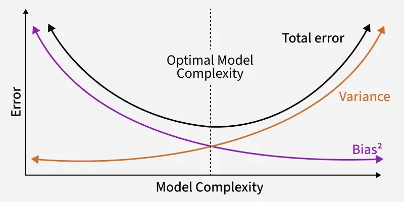
Bias-Variance tradeoff
**1. Bias:
- Error due to wrong assumptions in the learning algorithm.
- High bias means underfitting and model is too simple to capture patterns.
- Example: Linear model trying to fit highly non-linear data.
**2. Variance:
- Error due to model being too sensitive to small fluctuations in training data.
- High variance means overfitting and model performs well on training data but poorly on unseen data.
- Example: Deep decision tree memorizing training data.
**3. Tradeoff:
- Decreasing bias usually increases variance and vice versa.
- Our goal is to find a balance that minimizes total error.
\text{Total Error} = \text{Bias}^2 + \text{Variance} + \text{Irreducible Error}
26. What is Hyperparameter Tuning in Machine Learning?
Hyperparameter tuning is the process of finding the best set of hyperparameters for a machine learning model to maximize performance. Hyperparameters are parameters set before training like learning rate, number of trees in Random Forest, regularization strength, etc that cannot be learned directly from the data.
Common Hyperparameter Tuning Methods are:
- **Grid Search: It tries all possible combinations of hyperparameters from a predefined set. It is simple and exhaustive, but computationally expensive for large search spaces.
- **Random Search: Randomly samples combinations of hyperparameters are taken from a given range. Often faster than grid search and can find good results in **fewer iterations.
- **Bayesian Optimization: Builds a probabilistic model of the objective function and selects hyperparameters to maximize performance. Efficient for expensive models; balances exploration and exploitation.
27. What is Linear Regression? What are its Assumption?
Linear Regression is a supervised learning algorithm used to predict a continuous target variable based on one or more input features by fitting a linear relationship.
y=mx+c
Where:
- y = predicted output
- x = input feature
- m = slope (coefficient)
- c = intercept
**Assumptions of Linear Regression
- **Linearity: Relationship between x and y is linear.
- **Independence: Data points are independent.
- **Homoscedasticity: Error terms have constant variance.
- **Normality of Errors: Residuals follow a normal distribution.
- **No Multicollinearity: Features should not be highly correlated.
28. Explain how sigmoid function work in Logistic Regression and why it is not a Regrresion Model even though it name has it?
In logistic regression, we want to predict probabilities for binary outcomes (e.g., 0 or 1). The sigmoid function converts any real number into a value between 0 and 1, making it suitable for probabilities.
Sigmoid Equation:
\sigma(z) = \frac{1}{1 + e^{-z}}
- Despite the name, logistic regression is used for classification, not regression. As it does not predict continuous values like linear regression, but instead predicts probabilities.
- A threshold (e.g., 0.5) is applied to classify outcomes as 0 or 1.
**29. How to choose an optimal number of clusters?
- **Elbow Method: Plot the explained variance or within-cluster sum of squares (WCSS) against the number of clusters. The "elbow" point where the curve starts to flatten, indicates the optimal number of clusters.
- **Silhouette Score: Measures how similar each point is to its own cluster compared to other clusters. A higher silhouette score indicates better-defined clusters. The optimal number of clusters is the one with the highest average silhouette score.
- **Gap Statistic: Compares the clustering result with a random clustering of the same data. A larger gap between the real and random clustering suggests a more appropriate number of clusters.
30. What is Multicollinearity and Why is it a Problem?
Multicollinearity occurs when two or more independent features are highly correlated with each other in a dataset. This means one feature can be linearly predicted from another with high accuracy. It can cause problems like:
- **Unstable Coefficients: Makes regression coefficients unreliable and highly sensitive to small changes in data.
- **Interpretation Difficulty: Hard to determine the individual effect of each feature on the target variable.
- **Reduced Model Performance: May not affect prediction accuracy much, but impacts the explainability of the model.
- **Inflated Variance: Leads to high standard errors in coefficient estimates.
**Detection Methods:
- **Correlation Matrix: Check for high correlation between features.
- **Variance Inflation Factor (VIF): A VIF > 5 (or 10) usually indicates strong multicollinearity.
**Solution:
- Remove or combine correlated features.
- Use Principal Component Analysis (PCA) or other dimensionality reduction techniques.
- Apply regularization methods like Ridge regression.
31. What is Variance Inflation Factor?
The Variance Inflation Factor (VIF) is a statistical measure used to detect multicollinearity in regression models. It shows how much the variance of a regression coefficient is inflated because of correlation with other independent variables.
VIF_i = \frac{1}{1 - R_i^2}
Here R_i^2 is coefficient of determination when the i^{th} feature is regressed on all other features.
**Interpretation:
- **VIF = 1: No correlation with other features.
- **1 < VIF < 5: Moderate correlation, usually acceptable.
- **VIF > 5 (or 10): High multicollinearity i.e it is problematic and need to be resolved.
**32. What is Information Gain and Entropy in Decision Tree?
**1. Entropy
- Entropy is a measure of impurity or randomness in a dataset.
- If all samples belong to the same class → entropy = 0 (pure).
- If classes are equally mixed → entropy is high.
Entropy(S) = - \sum_{i=1}^{c} p_i \log_2(p_i)
Where:
- p_i = proportion of samples belonging to class iii
- c= number of classes
**2. Information Gain
- Information Gain measures the reduction in entropy when a dataset is split based on a feature.
- Higher information gain means the feature is better at splitting the data.
IG(S, A) = Entropy(S) - \sum_{v \in Values(A)} \frac{|S_v|}{|S|} \, Entropy(S_v)
Where:
- S= dataset
- A= feature used for split
- S_v = subset of S where feature A=v
**Relationship between Entropy and Information Gain:
- Entropy should be minimized i.e less impurity after splitting.
- Information Gain should be maximized i.e best feature chosen for splitting.
- Decision Trees always pick the feature with the highest Information Gain to reduce entropy the most.
**33. How to Prevent Overfitting in Decision Trees?
Decision trees are prone to overfitting because they can grow very deep and capture noise along with patterns. To prevent overfitting we can use following techniques:
- **Limit Tree Depth: Restrict max_depth so the tree doesn’t grow too complex.
- **Minimum Samples for Split/Leaf: Set min_samples_split or min_samples_leaf to ensure splits happen only when enough data is present.
- **Pruning: Remove branches that add little value (pre-pruning or post-pruning).
- **Feature Selection: Use only relevant features to avoid unnecessary splits.
- **Use Ensemble Methods: Techniques like Random Forest and Gradient Boosting average multiple trees to reduce variance.
- **Cross-Validation: Helps monitor performance on unseen data and avoid overly complex trees.
34. What is Pruning in Decision Trees?
Pruning is the process of removing unnecessary branches from a decision tree that do not provide significant predictive knowledge. It helps make the tree simpler, smaller and less overfitted. It improves generalization on unseen data and makes the model more interpretable and efficient. We have 2 types of pruning:
**1. Pre-Pruning (Early Stopping):
- Stop growing the tree early by setting constraints like max_depth, min_samples_split or min_samples_leaf.
- Prevents the tree from becoming too complex.
**2. Post-Pruning:
- Grow the full tree first, then remove branches that have little impact on accuracy.
- Example: Cost Complexity Pruning (CCP) balances tree accuracy and size using a penalty term.
35. Explain ID3 and CART
**1. ID3 (Iterative Dichotomiser 3): ID3 is a decision tree algorithm used only for classification. It uses Entropy and Information Gain to decide which feature should split the dataset. It works like:
- Calculate entropy of the dataset.
- For each feature, calculate information gain.
- Choose the feature with the highest information gain for the split.
- Repeat this process until all records are classified or stopping conditions are met.
**2. CART (Classification and Regression Trees): CART can be used for both classification and regression problems. It uses Gini Index for classification and Mean Squared Error (MSE) for regression. It works like:
- For each feature, calculate Gini Index (for classification) or MSE (for regression).
- Select the feature with the lowest impurity.
- Split the dataset into two branches (CART always creates binary trees).
- Repeat the process until stopping conditions are met.
| Feature | **ID3 | **CART |
|---|---|---|
| **Used for | Classification only | Classification & Regression |
| **Split Criterion | Information Gain (Entropy) | Gini Index (classification), MSE (regression) |
| **Output | Multi-way split possible | Always binary split (2 branches) |
| **Handling Data | Categorical mainly | Both numerical and categorical |
36. Explain Naive Bayes and Bayes’ Theorem.
Bayes’ Theorem calculates the probability of an event based on prior knowledge of related events.
P(A|B) = \frac{P(B|A) \cdot P(A)}{P(B)}
Where:
- P(A∣B): Posterior probability (probability of A given B).
- P(B∣A): Likelihood (probability of B given A).
- P(A): Prior probability of A.
- P(B): Evidence or probability of B.
Naive Bayes is a classification algorithm based on Bayes’ theorem. It assumes that all features are independent (naive assumption). It is widely used in weather forecast and classifying emails as spam or not spam. Its working is:
- Calculate prior probability of each class.
- Compute likelihood of features for each class.
- Apply Bayes’ theorem to get posterior probability.
- Assign the class with the highest posterior probability.
37. What are the assumptions of Naive Bayes?
Naive Bayes is based on a few key assumptions that simplify calculations:
- **Feature Independence: All features are assumed to be independent of each other given the class label.
- **All Features Contribute Equally: Each feature contributes equally and independently to the outcome.
- **Categorical or Conditional Probability: Features can be categorical or continuous, but for continuous data, it’s assumed to follow a probability distribution (like Gaussian).
- **Correctly Labeled Data: The training dataset is assumed to be accurately labeled, because incorrect labels affect probability estimates.
38. What are the types of Naive Bayes algorithm?
The main types of Naive Bayes algorithms are:
- **Gaussian Naive Bayes: Assumes continuous features follow a normal (Gaussian) distribution. Often used for features like height, weight or temperature.
- **Multinomial Naive Bayes: Works with discrete count data such as word counts in text classification (e.g., spam detection).
- **Bernoulli Naive Bayes: Suitable for binary features (0 or 1) like whether a word occurs in a document or not.
- **Categorical Naive Bayes: Used when features are categorical (like color: red, green, blue) rather than numeric.
39. Explain K-Nearest Neighbors (KNN) working.
K-Nearest Neighbors (KNN) is a supervised learning algorithm used for classification and regression. It predicts the output of a data point based on the majority class or average value of its K nearest neighbors. KNN is non-parametric algorithm and performance depends on K value and distance metric.
**How KNN works:
- Choose the number of neighbors KKK.
- Calculate the distance (e.g., Euclidean) between the new data point and all points in the training set.
- Select the K nearest neighbors based on distance.
- For classification, assign the most frequent class among neighbors. For regression, take the average value of neighbors.
40. Why is KNN a lazy algorithm?
K-Nearest Neighbors (KNN) is called a lazy learning algorithm because it does not learn an explicit model during training. Instead, it stores all training data and waits until a query (test data) is given to make predictions.
- No training phase and all computation happens at prediction time.
- Memory-intensive because it stores the entire training dataset.
- Simplicity makes it easy to implement but can be slow for large datasets.
41. How does the K value affect KNN?
A small K value makes KNN sensitive to noise and can lead to overfitting. A large K value smooths decision boundaries but can cause underfitting by ignoring local patterns. Choosing the right K balances overfitting and underfitting, often determined using cross-validation.
42. What are the different distance metrics in Machine Learning?
- **Euclidean Distance: Straight-line distance between two points in space.
- **Manhattan Distance: Sum of absolute differences of coordinates.
- **Minkowski Distance: Generalized form of Euclidean and Manhattan distances.
- **Cosine Similarity: Measures the cosine of the angle between two vectors (used for text or high-dimensional data).
- **Hamming Distance: Number of positions at which corresponding elements differ (used for categorical or binary data).
- **Mahalanobis Distance: Accounts for correlations between variables and useful for multivariate data.
43. How to find the optimal value of K in KNN?
Different techniques to find the optimal K include:
- **Cross-Validation: Test multiple K values using k-fold cross-validation and pick the one with the best validation performance.
- **Elbow Method: Plot error rate versus K and choose the K at the “elbow” point where error stabilizes.
- **Silhouette Score: Evaluate clustering quality (for KNN in clustering contexts) to select K with the best score.
- **Gap Statistic: Compare intra-cluster variation with a reference null distribution to choose K.
- **Grid Search: Systematically test a range of K values and select the best based on performance metrics.
- **Trial and Error: Manually test different K values and evaluate model accuracy (useful for small datasets).
**44. What is KNN Imputer and how does it work?
KNN Imputer fills missing values by referencing the k nearest neighbors of a data point based on a distance metric (e.g., Euclidean distance).
- **Neighborhood-based Imputation: Finds k closest points to the missing value.
- **Imputation: Uses the mean or median of neighbors to fill the missing value.
- **Distance Parameter: k defines how many neighbors are considered and the distance metric controls similarity.
45. What are the different distance metrics in Machine Learning?
Distance metrics measure how similar or dissimilar two data points are. They are widely used in clustering, K-NN and other ML algorithms. Different metrics work better depending on the type of data and problem. Common Distance Metrics:
**1. Euclidean Distance:
- Straight-line distance between two points in space.
- Most commonly used for continuous data.
**2. Manhattan Distance (L1 Norm):
- Sum of absolute differences between coordinates.
- Works well when you want to penalize differences equally across dimensions.
**3. Minkowski Distance:
- Generalization of Euclidean and Manhattan distances.
- Can be tuned with a parameter **p: p=1 → Manhattan, p=2 → Euclidean.
**4. Cosine Similarity / Cosine Distance:
- Measures the angle between two vectors, not magnitude.
- Useful for text data, document similarity or high-dimensional sparse data.
**5. Jaccard Distance:
- Measures dissimilarity between sets.
- Often used for binary or categorical features.
46. What is the decision boundary in SVM?
In Support Vector Machine (SVM), the decision boundary is the line (in 2D) or hyperplane (in higher dimensions) that separates data points of different classes. It is chosen so that the margin which is the distance between the hyperplane and the nearest data points, called support vectors is maximized. The decision boundary in SVM is the hyperplane that best separates the classes while maintaining the largest possible margin for better generalization.
47. Does SVM only work with linear data points?
No, SVMs are not limited to linear data. While a linear SVM works well when data is linearly separable, for non-linear data SVM uses the kernel trick. Kernels like polynomial, RBF or sigmoid transforms the data into a higher-dimensional space where a linear separation becomes possible.
48. What is the kernel trick?
The kernel trick in SVM is a technique that allows the algorithm to handle non-linear data by transforming it into a higher-dimensional space where it becomes linearly separable. Instead of explicitly computing the transformation, the kernel function computes the similarity between data points in the transformed space hence making the process efficient.
**Popular kernel functions in SVM:
- **Linear Kernel: Works well when the data is linearly separable or when the number of features is very large like text classification. It is fast and simple.
- **Polynomial Kernel: Useful when the relationship between features is non-linear but still polynomial in nature. Example: classifying data that follows circular or curved boundaries.
- **RBF (Radial Basis Function) Kernel / Gaussian Kernel: Best for highly complex and non-linear data where no clear linear boundary exists. It is the most commonly used kernel in practice.
- **Sigmoid Kernel: Behaves similarly to neural networks and can be used for certain datasets, but it is less common compared to RBF and polynomial kernels.
49. What is Ensemble Learning
Ensemble learning is a technique in Machine Learning where multiple models (often called weak learners) are combined to produce a stronger and more accurate model. Instead of relying on a single model, ensemble methods aggregate the predictions from several models to improve performance, reduce errors and handle overfitting.
**Different Techniques of Ensemble Learning:
- **Bagging (Bootstrap Aggregating): Builds several models on random subsets of data and averages their predictions. Example: Random Forest.
- **Boosting: Trains models sequentially where each new model focuses on correcting the errors of the previous ones. Example: AdaBoost, XGBoost.
- **Stacking: Trains multiple base models and combines predictions from multiple models using another model (meta-learner) to make the final prediction.
- **Voting: Combines results from different models and chooses the majority vote (for classification) or average (for regression).
50. Explain Bagging and Boosting.
1. **Bagging (Bootstrap Aggregating):
- Bagging trains multiple models in parallel using random subsets of the training data (with replacement).
- Each model gives a prediction and results are combined by majority voting (classification) or averaging (regression).
- It reduces variance and prevents overfitting.
- Example: Random Forest.
**2. Boosting:
- Boosting trains models sequentially where each new model focuses on correcting the mistakes of the previous ones.
- Models are combined by assigning higher weights to more accurate models.
- It reduces bias and improves accuracy but can overfit if not controlled.
- Examples: AdaBoost, Gradient Boosting, XGBoost.
51. What is Random Forest?
Random Forest is an ensemble learning method that builds multiple decision trees and combines their results to improve accuracy and stability. Instead of relying on a single decision tree, it takes the majority vote (for classification) or average (for regression) of many trees.
- Handles large datasets with higher accuracy than a single decision tree.
- Reduces overfitting by combining multiple trees.
- Works well with both categorical and numerical data.
- Provides feature importance, helping to understand which variables are most influential.
**How Random Forest Works:
- Creates multiple random subsets of the dataset using bootstrapping (sampling with replacement).
- Builds a decision tree for each subset, but at each node, it selects a random subset of features instead of using all features.
- Each tree makes a prediction independently.
- The final prediction is made by combining all tree outputs (majority voting for classification, average for regression).
52. What is Bootstrapping?
Bootstrapping is a sampling technique used in statistics and machine learning where we create multiple datasets by randomly selecting data points with replacement from the original dataset.
- "With replacement" means the same data point can appear multiple times in a new sample.
- Each bootstrap sample is usually the same size as the original dataset.
- It helps to estimate the variability and improve model stability by training on different random samples.
- Used in ensemble methods like Bagging and Random Forest to reduce variance and prevent overfitting.
**Example: If the dataset is [1, 2, 3, 4] tehn one bootstrap sample could be [2, 4, 2, 1] and another could be [3, 1, 4, 4].
**53. What are some of the hyperparameters of the random forest regressor which help to avoid overfitting?
The important hyperparameters of a Random Forest Regressor that help to control overfitting are:
- **max_depth: Restricts how deep a tree can grow. Smaller depth reduces complexity and prevents overfitting.
- **n_estimators: Number of trees in the forest. More trees usually improve stability, but too many just increase computation without reducing overfitting.
- **min_samples_split: Minimum samples required to split a node. Higher values prevent trees from creating overly specific splits.
- **min_samples_leaf: Minimum samples required at a leaf node. Larger values create smoother predictions and avoid capturing noise.
- **max_leaf_nodes: Limits the number of leaf nodes, thereby controlling tree growth and depth.
- **max_features: Number of features considered for splitting at each node. Using fewer features introduces randomness and helps reduce overfitting.
- **bootstrap: Whether to sample data with replacement for each tree. Bootstrapping introduces diversity in trees, reducing overfitting.
- **max_samples: If bootstrap is True, this defines how many samples are drawn to train each tree. Controlling this adds more randomness.
**54. Whether decision tree or random forest is more robust to outliers
Decision trees are somewhat sensitive to outliers, as extreme values can influence the splits. Random forests, being an ensemble of multiple decision trees, aggregate results from several trees which reduces the impact of outliers. Therefore, random forests are generally more robust to outliers compared to a single decision tree.
55. How does Random Forest ensure diversity among trees?
- **Bagging (Bootstrap Aggregating): Each tree is trained on a random subset of the data.
- **Feature Randomness: Each split considers a random subset of features, preventing trees from being identical.
56. Explain AdaBoost, XGBoost and CatBoost.
**1. AdaBoost (Adaptive Boosting)
- Works by combining multiple weak learners (usually shallow decision trees).
- Each new learner focuses more on the misclassified samples of the previous learners by assigning higher weights to them.
- Final prediction is a weighted majority vote (classification) or weighted sum (regression).
- **Best used when: You have simple models and want to improve them by focusing on difficult cases.
**2. XGBoost (Extreme Gradient Boosting)
- An optimized implementation of Gradient Boosting with high performance and regularization features.
- Builds trees sequentially where each new tree corrects errors of the previous ones by minimizing a differentiable loss function.
- Includes regularization terms (L1 and L2) to avoid overfitting.
- Highly efficient, parallelizable and widely used in competitions.
- **Best used when: You need fast, accurate models for structured/tabular data.
**3. CatBoost (Categorical Boosting)
- A gradient boosting algorithm designed to handle categorical features directly without needing extensive preprocessing like one-hot encoding.
- Uses ordered boosting to reduce prediction shift (bias caused by using the same data for building and training).
- Often requires less tuning and works well.
- **Best used when: Dataset has many categorical features and minimal preprocessing is preferred.
57. What is the difference between Gradient Boosting and CatBoost?
| Feature | Gradient Boosting | CatBoost |
|---|---|---|
| **Handling Categorical Data | Needs manual preprocessing like Label Encoding or One-Hot Encoding. | Handles categorical features natively, i.e no need for extra encoding. |
| **Boosting Type | Uses standard boosting where new models are trained sequentially on residuals. | Uses Ordered Boosting to prevent prediction shift (overfitting from using same data in training). |
| **Training Speed | Slower if dataset is large and categorical preprocessing is heavy. | Faster training for categorical-heavy datasets since encoding is avoided. |
| **Overfitting Control | May overfit if not tuned properly. | More robust against overfitting due to ordered boosting and symmetric trees. |
| **Best Use Case | General-purpose tabular datasets with numerical data. | Datasets with many categorical features (e.g., e-commerce, text-based or survey data). |
58. Explain K-Means Clustering
Clustering is an unsupervised learning technique where data is grouped into clusters such that:
- Points in the same cluster are more similar to each other.
- Points in different clusters are more dissimilar from each other.
K-Means is a popular clustering algorithm that divides the dataset into K clusters. Each cluster is represented by its centroid (average of all data points in that cluster). The goal is to minimize the distance of points from their cluster centroids. It is widely used in customer segmentation, image compression, anomaly detection and pattern recognition.
- It works well when clusters are spherical and well-separated.
- Sensitive to the initial placement of centroids.
- Requires predefining K which can be chosen using methods like Elbow Method or Silhouette Score.
- Can struggle with non-linear or overlapping clusters.
**How K-Means Works:
- Choose the number of clusters K.
- Randomly initialize K centroids.
- Assign each data point to the nearest centroid (cluster assignment).
- Recalculate centroids as the mean of all points in a cluster.
- Repeat steps 3–4 until centroids no longer change (convergence).
**Example: If K=3 and you feed customer purchase data, K-Means may group customers into 3 clusters like "low spenders" "medium spenders" and "high spenders."
**59. What is the concept of convergence in K-means?
Convergence occurs when centroids stabilize and data point assignments no longer change. Conditions for Convergence:
- Proper initialization (e.g., k-means++)
- Data naturally forms well-separated clusters
- Correct choice of number of clusters (k)
- Setting maximum iterations and tolerance for centroid changes
60. What is the advanced version of K-Means?
While K-Means is simple and widely used, it has limitations like sensitivity to outliers, need to predefine K and difficulty handling non-spherical clusters. Several advanced versions and alternatives improve upon it:
**1. K-Medoids (PAM – Partitioning Around Medoids):
- Instead of using the mean as the cluster center, it uses an actual data point (medoid).
- More robust to outliers compared to K-Means.
**2. K-Means++:
- An improved version of K-Means initialization.
- Chooses initial centroids more carefully which leads to better convergence and avoids poor clustering results.
**3. Mini-Batch K-Means:
- Uses small random samples (mini-batches) of data instead of the entire dataset.
- Much faster and scalable for large datasets.
**4. Fuzzy C-Means (Soft K-Means):
- Instead of hard assignment, each point has a probability of belonging to multiple clusters.
- Useful when clusters overlap.
61. Explain K-Means++ and Fuzzy C-Means
**1. K-Means++
- K-Means++ is an improved version of the standard K-Means algorithm.
- The main improvement is in centroid initialization i.e instead of picking centroids randomly, it chooses them far apart from each other.
- This reduces the chances of poor clustering and improves convergence speed.
- Works the same as K-Means after initialization: assigns points to the nearest centroid and updates centroids iteratively.
- **Best for: General clustering problems where standard K-Means may converge to a local minimum.
**2. Fuzzy C-Means (FCM)
- Fuzzy C-Means is a soft clustering algorithm, unlike K-Means which assigns points to one cluster only.
- Each data point has a membership probability for each cluster, ranging between 0 and 1.
- Centroids are computed based on weighted membership values of points.
- Useful when clusters overlap or when strict cluster boundaries are unrealistic.
- **Best for: Image segmentation, medical data or any scenario where a point can belong partially to multiple clusters.
62. What is Hierarchical Clustering?
Hierarchical clustering is an unsupervised clustering technique that builds a hierarchy of clusters, either by merging smaller clusters into bigger ones or splitting larger clusters into smaller ones. It produces a dendrogram which is a tree-like diagram showing the arrangement of clusters. Distance metrics (Euclidean, Manhattan) and linkage methods (single, complete, average) determine how clusters are merged or split.
Unlike K-Means, it does not require predefining the number of clusters. Types of Hierarchical Clustering:
**1. Agglomerative Clustering (Bottom-Up)
- It uses a bottom-up approach by merging small clusters into bigger ones.
- At each step, it merges the two closest clusters based on a chosen distance metric (e.g., Euclidean, Manhattan).
- The process continues until all points are merged into a single cluster or a stopping criterion is met.
- Produces a dendrogram showing how clusters are combined.
- **Pros: Easy to understand, no need to predefine number of clusters.
- **Cons: Can be computationally expensive for large datasets.
**2. Divisive Clustering (Top-Down)
- It is a top-down approach and it splits large clusters into smaller ones.
- At each step, it splits the cluster into smaller clusters based on dissimilarity.
- Continues splitting until each point forms its own cluster or a stopping criterion is met.
- Produces a dendrogram that can be cut at different levels to choose the number of clusters.
- **Pros: Can reveal the overall hierarchical structure clearly.
- **Cons: Rarely used in practice because it is more computationally intensive than agglomerative clustering.
63. Explain Linkage Methods in Hierarchical Clustering
In hierarchical clustering, linkage methods determine how the distance between clusters is calculated when merging or splitting them. The choice of linkage affects the shape and structure of the resulting clusters. Common Linkage Methods are:
**1. Single Linkage (Nearest Neighbor):
- Distance between two clusters = shortest distance between any two points, one from each cluster.
- Can result in “chaining effect” where clusters may become long and stretched.
**2. Complete Linkage (Furthest Neighbor):
- Distance between two clusters = largest distance between any two points, one from each cluster.
- Produces compact, tightly bound clusters, less sensitive to outliers.
**3. Average Linkage:
- Distance between two clusters = average distance between all pairs of points from both clusters.
- Balances the properties of single and complete linkage, producing moderately compact clusters.
**4. Centroid Linkage:
- Distance between clusters = distance between the centroids (mean points) of the clusters.
- Can handle larger datasets but may sometimes cause inversions in dendrograms.
**5. Ward’s Linkage:
- Merges clusters to minimize the total within-cluster variance.
- Produces clusters that are roughly equal in size and very compact.
64. Explain DBSCAN and OPTICS
**1. DBSCAN (Density-Based Spatial Clustering of Applications with Noise)
DBSCAN is a density-based clustering algorithm that groups together points that are closely packed in space and labels points in low-density regions as noise or outliers. It is particularly useful for discovering clusters of arbitrary shapes without needing to predefine the number of clusters. The algorithm relies on two key parameters:
eps(maximum distance for neighborhood points)minPts(minimum points required to form a dense region).
**Working of DBSCAN:
- Start with an unvisited point.
- If the point has at least
minPtswithin distanceeps, it becomes a core point and a new cluster starts. - Add all points density-reachable from the core point to the cluster.
- Repeat the process for all unvisited points until all points are either clustered or marked as noise.
**Advantages:
- Detects clusters of any shape.
- Identifies outliers/noise automatically.
- No need to predefine the number of clusters.
**Disadvantages:
- Sensitive to the choice of
epsandminPts. - Struggles with clusters of varying density.
- Computationally expensive for very large datasets.
**2. OPTICS (Ordering Points To Identify the Clustering Structure)
OPTICS is an extension of DBSCAN designed to handle clusters with varying densities. Instead of producing flat clusters, it creates an ordering of points based on reachability distances, allowing detection of clusters at different density levels. This produces a reachability plot which can be used to identify hierarchical cluster structures.
**Working of OPTICS:
- Compute the core distance for each point (distance to its
minPts-th neighbor). - Calculate the reachability distance from each point to its neighbors.
- Order points based on reachability distance to form a reachability plot.
- Identify clusters as valleys in the reachability plot representing dense regions.
**Advantages:
- Handles clusters with varying densities effectively.
- Can detect hierarchical structures of clusters.
- Identifies outliers/noise.
**Disadvantages:
- More computationally intensive than DBSCAN.
- Reachability plot interpretation can be complex for large datasets.
65. Explain GMM, DPMM and Affinity Propagation
**1. GMM (Gaussian Mixture Model)
GMM is a probabilistic clustering algorithm that assumes data points are generated from a mixture of several Gaussian distributions with unknown parameters. Unlike K-Means which assigns each point to a single cluster, GMM assigns a probability of belonging to each cluster. It is more flexible and can model elliptical clusters rather than only spherical ones.
**Working of GMM:
- Initialize parameters (means, covariances and mixing coefficients).
- Use the Expectation-Maximization (EM) algorithm to iteratively update.
- **E-step: Compute probabilities of each point belonging to each cluster.
- **M-step: Update parameters to maximize the likelihood based on these probabilities.
- Repeat until convergence.
**Advantages:
- Handles clusters with different shapes, sizes and orientations.
- Provides soft clustering, giving probabilities instead of hard assignments.
**Disadvantages:
- Requires specifying the number of clusters in advance.
- Sensitive to initialization and may converge to local optima.
**2. DPMM (Dirichlet Process Mixture Model)
DPMM is a non-parametric Bayesian clustering algorithm which is an extension of GMM. It does not require predefining the number of clusters. Instead, it uses a Dirichlet Process to allow the number of clusters to grow with the data.
**Working of DPMM:
- Start with a potentially infinite number of clusters.
- Assign data points probabilistically to existing clusters or create a new cluster based on the Dirichlet Process.
- Use Bayesian inference (e.g., Gibbs sampling) to update cluster assignments.
**Advantages:
- Automatically determines the optimal number of clusters.
- Handles complex and evolving datasets.
**Disadvantages:
- Computationally intensive due to Bayesian inference.
- More complex to implement and interpret compared to GMM.
**3. Affinity Propagation
Affinity Propagation is a message-passing clustering algorithm that identifies exemplars which are representative points for each cluster. Unlike K-Means or GMM, it does not require specifying the number of clusters.
**Working of Affinity Propagation:
- Initialize similarity scores between all pairs of points.
- Exchange responsibility and availability messages iteratively:
- **Responsibility: How suitable a point is as an exemplar for another point.
- **Availability: How appropriate it would be for a point to choose another point as its exemplar.
- After convergence, select exemplars and assign points to the nearest exemplar.
**Advantages:
- Automatically finds the number of clusters.
- Works well with non-spherical clusters.
- No need for initialization like K-Means.
**Disadvantages:
- High memory usage for large datasets due to similarity matrix.
- Slower for very large datasets.
66. Explain Association Rule Mining
Association Rule Mining is a data mining technique used to discover relationships or patterns among items in large datasets, particularly transactional data. It identifies rules that show how the presence of certain items in a transaction implies the presence of other items. It helps finding hidden patterns in large datasets and is useful for recommendations, cross-selling and promotions. It uses:
- **Support: Fraction of transactions that contain the itemset.
- **Confidence: Likelihood that the consequent occurs when the antecedent occurs.
- **Lift: Measures how much more often the antecedent and consequent occur together than expected if independent.
**Working Steps:
- Find frequent itemsets that meet a minimum support threshold using Apriori or FP-Growth.
- Generate association rules from these frequent itemsets that satisfy a minimum confidence threshold.
- Optionally, calculate lift to measure rule strength.
**Example: Suppose a small grocery dataset has transactions:
| Transaction ID | Items Bought |
|---|---|
| 1 | Milk, Bread |
| 2 | Milk, Diaper, Beer |
| 3 | Bread, Diaper, Milk |
| 4 | Bread, Beer |
- **Rule: {Milk, Bread} → {Diaper}
- **Support: 1/4 = 25% (1 transaction contains all three items)
- **Confidence: 1/2 = 50% (2 transactions contain Milk and Bread, only 1 also contains Diaper)
- **Lift: Confidence / Support of Diaper = 0.5 / 0.5 = 1
67. Explain Apriori Algorithm and FP-Growth Algorithm
**1. Apriori Algorithm
Apriori is a classic algorithm for association rule mining. It identifies frequent itemsets in transactional datasets and generates strong rules based on minimum support and confidence thresholds.
**Working Steps:
- Scan the dataset to find all frequent 1-itemsets that meet the minimum support.
- Generate candidate 2-itemsets from the frequent 1-itemsets and count their occurrences.
- Repeat the process to generate k-itemsets until no more frequent itemsets can be found.
- From frequent itemsets, generate association rules that satisfy minimum confidence.
**2. FP-Growth Algorithm (Frequent Pattern Growth)
FP-Growth is an efficient alternative to Apriori. Instead of generating candidate itemsets, it uses a compressed data structure called FP-Tree to store transactions.It is faster than Apriori for large datasets and requires fewer scans of the dataset. It handles large transaction datasets efficiently.
**Working Steps:
- Build an FP-Tree by scanning the dataset once to store frequent items in a compact tree structure.
- Recursively extract frequent itemsets from the FP-Tree using a divide-and-conquer approach.
- Generate association rules from the frequent itemsets.
68. Explain Content-Based and Collaborative Filtering Recommendation Systems
**1. Content-Based Filtering: It recommends items to a user based on the features of items they have liked in the past. It analyzes item attributes like genre, category, keywords or specifications and matches them with the user’s preferences.
- Can recommend items without knowing item features.
- Can provide serendipitous recommendations that are different from what the user already knows.
- Struggles with cold start problem (new users or new items).
- Requires large user interaction data to be effective.
**Working:
- Represent items using a feature vector.
- Compare the feature vectors of new items with items the user liked using similarity metrics (e.g., cosine similarity).
- Recommend items with the highest similarity scores.
For example, a user watches movies with action and sci-fi genres. The system recommends other action or sci-fi movies based on these features.
**2. Collaborative Filtering: It recommends items based on user behavior and interactions, rather than item features. It assumes that users with similar tastes in the past will like similar items in the future.
- Can recommend items without knowing item features.
- Can provide serendipitous recommendations that are different from what the user already knows.
- Struggles with cold start problem (new users or new items).
- Requires large user interaction data to be effective.
**Working:
- **User-Based CF: Finds users similar to the target user and recommends items they liked.
- **Item-Based CF: Finds items similar to those the user liked and recommends them.
For example, user A and user B both liked movies X and Y. User A liked movie Z, so movie Z is recommended to User B.
69. Explain the EM Algorithm
The Expectation-Maximization (EM) algorithm is a statistical technique used to find maximum likelihood estimates of parameters in models with latent (hidden) variables. It is widely used in clustering like Gaussian Mixture Models, missing data imputation and probabilistic models.
- Can handle missing or incomplete data.
- Works well for probabilistic models and mixture models.
- Can converge to local maxima instead of the global maximum which can cause a problem.
- Sensitive to initial parameter values.
The EM algorithm works iteratively in two main steps:
**1. Expectation Step (E-step):
- Estimate the probability that each data point belongs to each cluster (or hidden state) using the current parameters.
- Essentially, calculate expected values of the latent variables given the observed data.
**2. Maximization Step (M-step):
- Update the model parameters to maximize the likelihood using the probabilities calculated in the E-step.
- This step refines estimates of parameters like means, variances and mixture coefficients in clustering.
**3. Repeat the E-step and M-step until the parameters converge or the likelihood improvement is below a threshold.
70. Explain Markov Model and Hidden Markov Model (HMM)
**1. Markov Model (MM): A Markov Model is a probabilistic model that represents a system which moves between states with certain probabilities. The key property is the Markov property which states that the next state depends only on the current state, not on the past history.
- Simple and mathematically tractable.
- Useful for modeling sequential data where future depends only on present.
- Cannot model systems where the next state depends on more than just the current state.
**Working:
- Define a set of states.
- Define transition probabilities between states.
- Predict the next state based on the current state using these probabilities.
Example****:** Weather prediction: If today is **sunny, the probability that tomorrow is sunny or rainy depends only on **today’s weather, not on previous
**2. Hidden Markov Model (HMM): It is an extension of Markov Model where the states are hidden (not directly observable) and we only observe emissions or outputs that depend probabilistically on these hidden states.
- Can model sequential data with hidden processes.
- Widely used in speech recognition, bioinformatics and NLP.
- Requires training to estimate transition and emission probabilities.
- Computationally more complex than basic Markov Models.
**Working:
- Define hidden states and observable outputs.
- Define transition probabilities between hidden states and emission probabilities from states to observations.
- Use algorithms like Forward-Backward or Viterbi to infer hidden states from observed data.
Example: In speech recognition the actual phonemes (hidden states) are not observed, but the audio signal (observations) is observed. HMM predicts the sequence of phonemes from the signal.
71. Explain PCA (Principal Component Analysis)
Principal Component Analysis (PCA) is a dimensionality reduction technique used in machine learning and statistics. It transforms a high-dimensional dataset into a lower-dimensional space while preserving as much variance (information) as possible. PCA is widely used for visualization, noise reduction and feature extraction.
- Reduces computational complexity by lowering dimensions.
- Removes redundant or correlated features.
- Helps in visualizing high-dimensional data.
- Principal components may lack interpretability.
- Assumes linear relationships between features.
- Sensitive to scaling of features and standardization is necessary.
**Working of PCA:
- Standardize the data to have mean 0 and variance 1.
- Compute the covariance matrix of the features.
- Calculate the eigenvalues and eigenvectors of the covariance matrix.
- Eigenvectors define the directions (principal components).
- Eigenvalues indicate the amount of variance in each direction.
- Select top k principal components with the highest eigenvalues.
- Transform the original data onto the new k-dimensional space.
**Example:
- Dataset with features like height, weight, age and income.
- PCA can reduce it to 2 or 3 principal components that capture most of the variance for visualization or modeling.
**72. Why does PCA maximize variance in the data?
PCA focuses on directions with highest variance, as variance represents information content. By projecting data onto these directions:
- Information is preserved while reducing dimensionality.
- Less important features with low variance are discarded, simplifying the data.
73. Explain NMF, LDA and t-SNE
**1. NMF (Non-Negative Matrix Factorization): NMF is a dimensionality reduction and feature extraction technique where a non-negative matrix is factorized into two lower-rank non-negative matrices. It is often used for topic modeling, image processing and recommendation systems.
- Produces interpretable components since values are non-negative.
- Useful in text mining and image decomposition.
- Sensitive to initialization.
- May converge to local minima.
**Working:
- Input matrix V (e.g., document-term matrix) is approximated as V \approx W \cdot H where W and H are non-negative matrices.
- W represents basis features and H represents coefficients for reconstructing the original data.
- Iteratively update W and H to minimize reconstruction error.
**2. LDA (Latent Dirichlet Allocation): LDA is a probabilistic topic modeling algorithm used to discover hidden topics in a collection of documents. Each document is represented as a mixture of topics and each topic is a distribution over words.
- Discovers hidden thematic structures in large text corpora.
- Can handle unlabeled data effectively.
- Assumes bag-of-words, ignoring word order.
- Choosing the number of topics is often subjective.
**Working:
- Assign each word in a document to a topic randomly initially.
- Iteratively update topic assignments using Dirichlet priors to maximize the likelihood of observed words.
- After convergence, output: topic distribution per document or word distribution per topic.
**3. t-SNE (t-Distributed Stochastic Neighbor Embedding): It is a non-linear dimensionality reduction technique mainly used for visualizing high-dimensional data in 2D or 3D space. It preserves local structure (similar points stay close) while reducing dimensions.
- Excellent for visualizing clusters in high-dimensional data.
- Preserves local neighborhoods well.
- Computationally expensive for large datasets.
- Does not preserve global distances.
- Results can vary depending on perplexity and initialization.
**Working:
- Compute pairwise similarities between points in high-dimensional space.
- Define similarities in lower-dimensional space.
- Minimize Kullback-Leibler divergence between the two distributions using gradient descent.
74. Explain Manifold Learning and Its Techniques
Manifold Learning is a non-linear dimensionality reduction technique used to uncover the low-dimensional structure (manifold) embedded in high-dimensional data. The idea is that high-dimensional data often lies on a lower-dimensional manifold and learning this structure helps in visualization, feature extraction and noise reduction. Key Techniques in Manifold Learning:
**1. Isomap (Isometric Mapping):
- Preserves the geodesic (shortest path) distances between points on the manifold.
- Good for unfolding non-linear structures in high-dimensional data.
- Example: Mapping a Swiss roll dataset to a flat 2D plane.
**2. Locally Linear Embedding (LLE):
- Preserves local relationships among neighboring points.
- Each point is expressed as a linear combination of its neighbors, then projected to a lower-dimensional space while preserving these relationships.
- Works well when data lies on a smooth manifold.
**3. t-SNE (t-Distributed Stochastic Neighbor Embedding):
- Focuses on preserving local neighborhoods while reducing dimensions for visualization.
- Maps similar points close together in 2D or 3D for cluster visualization.
**4. UMAP (Uniform Manifold Approximation and Projection):
- Preserves both local and some global structures.
- Faster than t-SNE for large datasets and useful for visualizing clusters.
**5. Multidimensional Scaling (MDS):
- Preserves pairwise distances between points while reducing dimensions.
- Can work for both linear and non-linear data depending on distance metric.
75. Explain Time Series Analysis and Forecasting
Time Series Analysis is the study of data points collected sequentially over time. It focuses on understanding patterns, trends, seasonality and other temporal structures in data. Common applications include stock prices, weather data, sales trends and sensor readings.
Forecasting is the process of predicting future values based on historical time series data. Time series forecasting helps in decision-making, resource planning and trend prediction.
- Captures temporal patterns and dependencies in data.
- Helps in planning, inventory management and forecasting future trends.
- Requires large historical data for accurate predictions.
- Sensitive to outliers and sudden changes in data.
- Modeling seasonality and trends can be complex.
**Key Components of Time Series:
- **Trend: Long-term increase or decrease in data (e.g., yearly sales growth).
- **Seasonality: Repeating patterns at fixed intervals (e.g., monthly or yearly).
- **Cyclic Patterns: Fluctuations without fixed periodicity (e.g., economic cycles).
- **Noise: Random variations or irregular fluctuations.
76. Explain ARIMA and SARIMA Models
**1. ARIMA (AutoRegressive Integrated Moving Average): It is a popular statistical model for time series forecasting, especially when the data is non-stationary. It combines three components:
- **AR (AutoRegressive): Uses past values of the series to predict the current value.
- **I (Integrated): Uses differencing to make the series stationary (remove trends).
- **MA (Moving Average): Uses past forecast errors to improve prediction.
**Notation: ARIMA(p, d, q)
- **p: Number of lag observations in AR component.
- **d: Degree of differencing to make series stationary.
- **q: Number of lagged forecast errors in MA component.
**Advantages:
- Effective for non-stationary time series.
- Captures trend and autocorrelation in data.
**Disadvantages:
- Assumes linear relationships.
- Does not handle seasonality directly.
**Example: ARIMA forecasting monthly sales of a product without strong seasonality.
**2. SARIMA (Seasonal ARIMA): It extends ARIMA to handle seasonal effects in time series. It includes seasonal components along with non-seasonal ARIMA components.
**Notation: SARIMA(p, d, q)(P, D, Q, m)
- **p, d, q: Non-seasonal ARIMA parameters.
- **P, D, Q: Seasonal AR, differencing and MA parameters.
- **m: Number of periods in a season (e.g., 12 for monthly data with yearly seasonality).
**Advantages:
- Handles both trend and seasonality.
- Widely used for seasonal sales, weather and demand forecasting.
**Disadvantages:
- More complex to tune than ARIMA.
- Requires enough seasonal data for accurate modeling.
**Example: SARIMA forecasting electricity demand which shows yearly seasonal patterns.
77. Explain Exponential Smoothing in Time Series
Exponential Smoothing is a time series forecasting method that gives more weight to recent observations while gradually decreasing the weight for older observations. It is widely used for short-term forecasting because it reacts quickly to changes in data.
- Simple and computationally efficient.
- Reacts quickly to recent changes in the data.
- Works well for short-term forecasting.
- Not ideal for complex patterns with irregular fluctuations.
- Requires careful tuning of smoothing parameters.
For example, Predicting next month’s sales based on recent monthly sales, giving higher weight to the last few months.
Types of Exponential Smoothing are:
**1. Simple Exponential Smoothing (SES):
- Used for data without trend or seasonality.
- Forecast is a weighted average of past observations, with weights decreasing exponentially for older data.
- Formula: F_{t+1} = \alpha \cdot Y_t + (1 - \alpha) \cdot F_t
- Here α (alpha) is Smoothing factor between 0 and 1.
**2. Holt’s Linear Exponential Smoothing:
- Used for data with trend but no seasonality.
- Extends SES by adding a trend component.
- Forecast formula: F_{t+h} = L_t + h \cdot T_t
- Here L_t is Level at time t and T_t Trend at time t.
**3. Holt-Winters Exponential Smoothing:
- Used for data with trend and seasonality.
- Can be additive (seasonal effect is constant) or multiplicative (seasonal effect changes proportionally).
- Forecast formula (additive):
- Here S is Seasonal component and m is Season length.
78. What is the concept drift in ML?
Concept drift refers to the change in the statistical properties of data (input or target variable) over time which causes a trained model to become less accurate because it was built on old data patterns.
**Example: A spam detection model trained on last year’s emails may fail when spammers change their techniques this year.
**Types of Concept Drift:
- **Sudden Drift: The data distribution changes abruptly.
- **Gradual Drift: The change happens slowly over time.
- **Recurring Drift: Old patterns reappear after some time.
**Handling Concept Drift:
- Regularly retraining the model with new data.
- Using adaptive learning algorithms that update as new data arrives.
79. What is Reinforcement Learning?
Reinforcement Learning (RL) is a type of machine learning where an agent learns to make decisions by interacting with an environment. The agent takes actions, receives feedback in the form of rewards or penalties and adjusts its behavior to maximize long-term rewards.
- **Agent: The learner or decision-maker.
- **Environment: The system the agent interacts with.
- **State: Current situation of the agent in the environment.
- **Action: Choice made by the agent.
- **Reward: Feedback signal for the action taken.
- **Policy: Strategy that defines the agent’s actions in given states.
**Example:
- A robot learning to walk.
- A self-driving car deciding when to stop or accelerate.
- A game-playing AI improves its moves through trial and error.
RL is about learning by trial and error with feedback, aiming to maximize cumulative rewards over time.
80. What is a Markov Decision Process (MDP)?
A Markov Decision Process (MDP) is a mathematical framework used in Reinforcement Learning to model decision-making situations where outcomes are partly random and partly under the control of an agent. It provides a structured way to describe environments in terms of states, actions, rewards and transitions, assuming the Markov property i.e the future state depends only on the current state and action, not on past states.
**Components of MDP:
- **States (S): All possible situations the agent can be in.
- **Actions (A): Choices available to the agent at each state.
- **Transition Probability (P): Probability of moving from one state to another given an action.
- **Reward (R): Immediate feedback received after taking an action.
- **Policy (π): A strategy mapping states to actions.
An MDP formalizes the environment in RL, helping the agent learn an optimal policy that maximizes expected rewards over time.
**Example: In a grid-world game, each cell is a state, moving up/down/left/right are actions, rewards could be points gained or lost and transitions depend on the action taken.
81. What is an Optimal Policy?
In Reinforcement Learning, an optimal policy is the strategy that maps states to actions that maximizes the expected cumulative reward for an agent over time.
- A policy (π) defines what action an agent should take in each state.
- An optimal policy (π*) ensures that no other policy can achieve a higher long-term reward.
**Example: In a self-driving car scenario:
- A normal policy may tell the car to "usually stop at red lights."
- The optimal policy always ensures the car stops at red lights to avoid accidents.
**82. What is the Bellman Equation in Reinforcement Learning?
The Bellman Equation is a fundamental recursive relationship in Reinforcement Learning that expresses the value of a state in terms of the rewards and the value of its successor states. It provides a way to break down the long-term return into immediate reward plus the discounted value of future states.
- Defines how values are updated recursively.
- Foundation for algorithms like Value Iteration and Q-Learning.
- Helps in finding the optimal policy by balancing immediate and future rewards.
Mathematically, for a state-value function ( V(s) ): V(s) = \mathbb{E}[R_{t+1} + \gamma V(S_{t+1}) \mid S_t = s]
Where:
- V(s): Value of state ( s )
- R_{t+1}: Reward received after taking an action
- \gamma : Discount factor (0 ≤ γ < 1)
- S_{t+1}: Next state
For action-value function ( Q(s,a) ): Q(s,a) = \mathbb{E}[R_{t+1} + \gamma \max_{a'} Q(S_{t+1}, a') \mid S_t = s, A_t = a]
**83. What is Dynamic Programming (DP) in Reinforcement Learning?
Dynamic Programming (DP) in RL is a group of algorithms that solve Markov Decision Processes (MDPs) using the Bellman equations, assuming the environment’s dynamics (transition probabilities and rewards) are fully known.
- Based on the principle of optimality i.e optimal solutions can be built from subproblems.
- Uses methods like policy evaluation, policy iteration and value iteration.
- Provides a foundation for many RL algorithms but is not practical for real-world problems where the model is unknown.
- Works best in small, finite environments with complete knowledge of state transitions.
In short DP is a planning method in RL that computes optimal policies using exact models of the environment.
84. Explain Value Iteration and Policy Iteration in Reinforcement Learning.
Both Value Iteration and Policy Iteration are Dynamic Programming methods used to find the optimal policy in a Markov Decision Process (MDP).
**1. Value Iteration: Directly computes the optimal value function by repeatedly applying the Bellman Optimality Equation. It iteratively improves state values until they stabilize, then extracts the best policy.
Update rule: V_{k+1}(s) = \max_a \sum_{s'} P(s' \mid s,a) [R(s,a,s') + \gamma V_k(s')]
After convergence, the optimal policy is derived as: \pi^*(s) = \arg\max_a \sum_{s'} P(s' \mid s,a) [R(s,a,s') + \gamma V(s')]
**2. Policy Iteration: It improves the policy step by step, guaranteeing convergence to the optimal policy in finite MDPs. Alternates between two steps are:
- Policy Evaluation: Compute value function for the current policy.
- Policy Improvement: Update the policy using the new value function.
Repeat until the policy no longer changes (converges to optimal policy).
**Comparison:
- **Value Iteration: Faster in practice, directly approximates the optimal value.
- **Policy Iteration: More systematic, but requires solving policy evaluation multiple times.
**85. Explain Model-Free RL and Model-Based RL.
In Reinforcement Learning, methods are broadly divided into Model-Free and Model-Based approaches, depending on whether the agent has access to the environment’s dynamics.
**1. Model-Free RL
- The agent learns directly from experience without knowing transition probabilities or reward functions.
- Relies on trial-and-error to estimate value functions or policies.
- **Examples: Q-Learning, SARSA, Deep Q-Networks (DQN).
No environment model needed hence it learns purely from interactions.
**2. Model-Based RL
- The agent tries to learn or use a model of the environment (state transitions and rewards).
- Uses the model for planning by simulating future states and rewards.
- Examples: Dyna-Q, Monte Carlo Tree Search (MCTS).
It needs a model of the environment and can plan ahead before acting.
**Comparison:
- **Model-Free: Easier to implement, works in unknown environments, but often sample-inefficient.
- **Model-Based: More sample-efficient, allows planning, but requires learning/knowing a model which may be complex.
**86. Explain Q-Learning and Deep Q-Learning.
**1. Q-Learning
- A model-free, off-policy RL algorithm that learns the value of taking an action in a state.
- It updates an action-value function ( Q(s,a) ) using the Bellman equation.
Update rule: Q(s,a) \leftarrow Q(s,a) + \alpha \big[R + \gamma \max_{a'} Q(s',a') - Q(s,a)\big]
Where:
- \alpha : Learning rate
- R : Reward received
- \gamma : Discount factor
- s' : Next state
- a' : Next action
Learns optimal policy by updating Q-values through repeated interactions.
**2. Deep Q-Learning (DQN)
- An extension of Q-Learning where a neural network approximates the Q-function instead of using a Q-table.
- Useful when state space is very large or continuous.
- Introduced techniques to improve stability that are:
- **Experience Replay: Store past experiences and sample randomly to break correlation.
- **Target Network: Use a separate network to compute stable target values.
Scales Q-Learning to high-dimensional problems using deep neural networks.
**Comparison:
- **Q-Learning: Works for small, discrete state-action spaces.
- **Deep Q-Learning: Handles complex environments with large/continuous state spaces.
**87. Explain SARSA in Reinforcement Learning.
SARSA (State–Action–Reward–State–Action) is a model-free, on-policy RL algorithm that learns the action-value function Q(s,a). Unlike Q-Learning, which is off-policy, SARSA updates values based on the current policy’s action rather than the greedy action.
- On-policy i.e it learns using the action actually taken by the current policy.
- More conservative than Q-Learning, as it considers exploratory actions.
- Often safer in risky environments since it doesn’t assume greedy action selection.
Update rule:Q(s,a) \leftarrow Q(s,a) + \alpha \big[R + \gamma Q(s',a') - Q(s,a)\big]
Where:
- s: Current state
- a : Current action (taken by the policy)
- R : Reward received
- s' : Next state
- a' : Next action chosen by the same policy
- \alpha : Learning rate
- \gamma : Discount factor
**88. What is the difference between Q-Learning and SARSA?
| Feature | Q-Learning | SARSA |
|---|---|---|
| Learning type | Off-policy (learns from greedy action) | On-policy (learns from action actually taken) |
| Policy used | Updates values assuming the best action is chosen next | Updates values based on the policy’s chosen next action |
| Exploration impact | Ignores exploratory moves in update | Accounts for exploratory moves in update |
| Behavior | More aggressive, aims for optimal policy faster | More conservative, safer in risky environments |
**89. Explain Policy Gradient Methods in Reinforcement Learning.
Policy Gradient methods are a family of RL algorithms that directly optimize the policy (probability distribution over actions) instead of learning value functions. They adjust policy parameters using gradient ascent to maximize expected cumulative reward.
- Instead of deriving a policy from value functions, the policy is represented as \pi_\theta(a|s) with parameters \theta.
- The parameters are updated in the direction of the gradient of expected reward: \theta \leftarrow \theta + \alpha \nabla_\theta J(\theta)
Where:
- J(\theta) : Objective function (expected return)
- \alpha : Learning rate
**Advantages:
- Works well in continuous action spaces.
- Can represent stochastic policies.
- More flexible than value-based methods.
**Examples of Policy Gradient methods:
- REINFORCE algorithm (Monte Carlo Policy Gradient).
- Actor-Critic methods (combine policy gradient with value function).
**90. Explain the REINFORCE Algorithm and Actor-Critic Methods in Reinforcement Learning.
**1. REINFORCE Algorithm (Monte Carlo Policy Gradient): A policy gradient method that updates the policy parameters using complete episode returns. The policy is parameterized as \pi_\theta(a|s). It is:
- Simple to implement.
- High variance since it waits for full episode returns.
- Works better with baseline subtraction to reduce variance.
Update rule: \theta \leftarrow \theta + \alpha , G_t , \nabla_\theta \log \pi_\theta(a_t|s_t)
Where:
- G_t : Total discounted return after time ( t )
- \alpha : Learning rate
- \nabla_\theta \log \pi_\theta(a_t|s_t) : Gradient of log probability of the taken action
**2. Actor-Critic Methods: It combines **policy-based (actor) and **value-based (critic) methods. It is useful for:
- Lower variance than REINFORCE since critic gives step-by-step feedback.
- More efficient in large/continuous state spaces.
- Forms the basis of modern RL algorithms (e.g., A2C, PPO).
Here:
- **Actor: Updates the policy parameters (like in policy gradient).
- **Critic: Estimates the value function to provide feedback (baseline) for the actor.
Update rule:
- **Actor update: \theta \leftarrow \theta + \alpha , \delta_t , \nabla_\theta \log \pi_\theta(a_t|s_t)
- **Critic update: w \leftarrow w + \beta , \delta_t , \nabla_w V_w(s_t)
**Comparison:
- **REINFORCE: Pure policy gradient, simple but high variance.
- **Actor-Critic: Hybrid approach, reduces variance using value function guidance.
**91. What is Monte Carlo Policy Gradient in Reinforcement Learning?
Monte Carlo Policy Gradient refers to RL methods that update policy parameters using complete returns from full episodes, rather than bootstrapping from intermediate states. Monte Carlo Policy Gradient methods directly adjust the policy using complete episode returns, forming the foundation of REINFORCE.
- Uses the total **discounted return ( G_t ) of an episode to update the policy.
- Simple to implement but has **high variance, as updates depend on the full episode outcome.
- Often combined with **baseline subtraction or variance-reduction techniques to improve stability.
Policy is represented as \pi_\theta(a|s) and parameters are updated using: \theta \leftarrow \theta + \alpha , G_t , \nabla_\theta \log \pi_\theta(a_t|s_t)
**92. What is Proximal Policy Optimization (PPO) in Reinforcement Learning?
Proximal Policy Optimization (PPO) is a state-of-the-art policy gradient method that improves training stability by limiting how much the policy is updated at each step. It is widely used in continuous and high-dimensional action spaces.
- PPO uses a surrogate objective to maximize expected reward while constraining policy updates.
- Balances exploration and policy stability.
- Easier to tune than older methods like TRPO.
- Forms the basis of many modern RL implementations (e.g., OpenAI Gym, robotics, game-playing agents).
It prevents large updates that could destabilize learning by clipping probability ratios: L^{CLIP}(\theta) = \mathbb{E}_t \Big[\min\big(r_t(\theta) \hat{A}_t, \text{clip}(r_t(\theta), 1-\epsilon, 1+\epsilon) \hat{A}_t\big)\Big]
Where:
- r_t(\theta) = \frac{\pi_\theta(a_t|s_t)}{\pi_{\theta_{old}}(a_t|s_t)} : Probability Ratio
- \hat{A}_t : Advantage estimate
- \epsilon : Clip parameter
PPO updates policies cautiously to improve performance while avoiding catastrophic policy changes.